From Molecules to Compositions

Bayesian Compositional Models for Sequencing Data

Seong-Hwan Jun

Department of Biostatistics and Computational Biology, University of Rochester Medical Center

From biological questions to statistical models

What is biostatistics?

Biostatistics develops statistical models and methods for learning about biological and health systems from imperfect measurements.

\[ \text{scientific question} \rightarrow \text{measurement process} \rightarrow \text{statistical model} \rightarrow \text{inference} \]

Why statistical inference?

Biological data vary for several reasons:

Technical variability: repeated measurements of the same biological material may produce different sequencing counts.
Biological variability: cells, tissues, and individuals genuinely differ in their molecular abundance.
Population variability: even within the same disease or treatment group, individuals are not identical.

Statistical inference = Probabilistic modeling + Observed data.

A probabilistic model describes how these sources of variation generate the observed data.

Observed data allow us to estimate the unknown parameters of a probabilistic model.

As the sample size increases, random variation averages out, uncertainty decreases, and we become more confident about systematic biological differences.

But inference is only meaningful after we define the biological quantity we want to learn.

Biological systems come in many forms

Biostatistics may study:

Molecular systems

genes and transcripts
messenger RNA
microRNAs
proteins and metabolites

Microbial ecosystems

microbial taxa
microbial genes
community functions
host–microbiome interactions

Different biological systems can produce remarkably similar statistical measurement problems.

What changes in disease?

Disease changes biological systems, not isolated variables.

Which genes, microRNAs, microbial taxa, or pathways change?
Are these isolated changes, or coordinated biological programs?
Which changes are direct, and which are induced by changes elsewhere in the system?

RNA biology: molecules as biological signals

Central dogma of biology (information flow):

\[ \text{DNA} \Rightarrow \underbrace{\text{RNA}} \Rightarrow \text{Protein} \Rightarrow \text{Cellular function}. \]

RNA abundance reflects:

transcriptional regulation
cell identity and cell state
stress and immune response
disease processes
tissue and cell-type composition

From biological abundance to RNA-seq counts

Tissue/cells $\Rightarrow$ RNA extraction $\Rightarrow$ library preparation $\Rightarrow$ sequencing $\Rightarrow$ read counts.

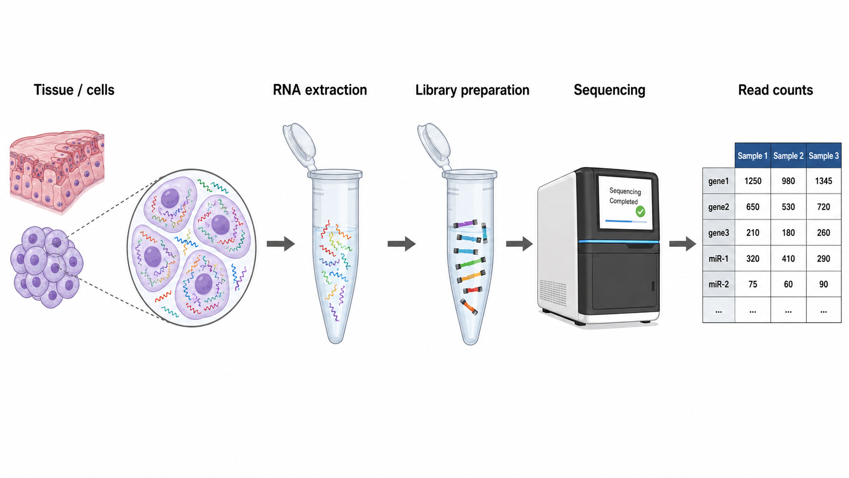
RNA-seq workflow from tissue and cells to read counts

From biological abundance to RNA-seq counts

RNA molecules are extracted from each sample (e.g., patient).
Target different types of RNA using different library preparation protocols (e.g., messenger RNA, microRNA, rRNA, tRNA).
Sequencing produces read counts for genes, transcripts, microRNAs, and other molecular features.

These counts are imperfect measurements shaped by both biology and the sequencing process.

Ways to measure RNA molecules

Assay	What is measured	Main question
Bulk mRNA-seq	Messenger RNA pooled across many cells	Which genes are expressed differently across samples or conditions?
Total RNA-seq	Coding and noncoding RNA pooled across many cells	How does the broader transcriptome change?
Single-cell RNA-seq	RNA from individual cells	Which cell types and cell states are present, and how do they differ?
Single-nucleus RNA-seq	Nuclear RNA from individual nuclei	How does gene expression vary across cells in tissues that are difficult to dissociate? e.g., brain.
Spatial transcriptomics	RNA abundance together with tissue location	Where are genes expressed within the tissue?
Small RNA-seq	miRNAs and other short RNAs	Which regulatory small RNAs are present and differentially abundant?
Long-read RNA sequencing	Full-length RNA molecules and transcript isoforms	Which transcript isoforms and splice variants are expressed?

Microbial communities as ecosystems

The human microbiome consists of communities of microorganisms—including bacteria, archaea, fungi, and viruses—that live in and on the body.

These communities interact with one another and with the host. They can:

help digest dietary components that human cells cannot process alone
produce metabolites and vitamins
influence immune-system development and regulation
protect against colonization by harmful organisms

The host and its microbiome form an interconnected biological system.

Diet, antibiotics, infection, inflammation, and disease may alter individual microorganisms as well as the structure and function of the entire community.

Case study: restoring a disrupted microbial ecosystem

van Nood et al (2013).

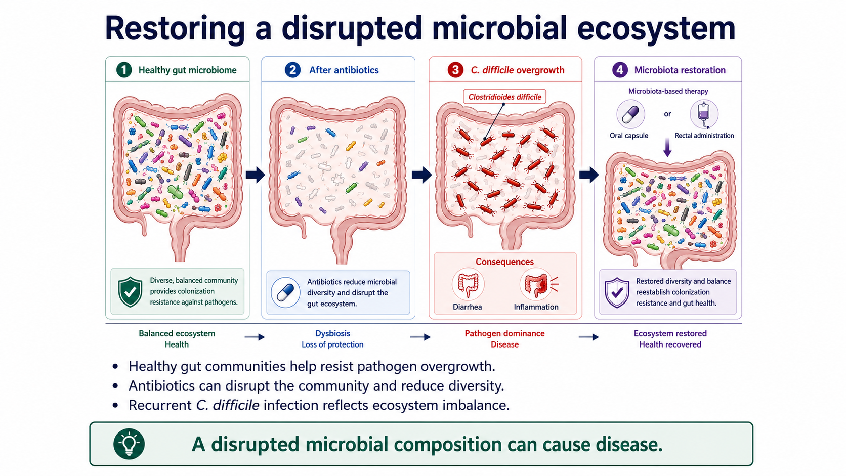
Case study: restoring a disrupted microbial ecosystem

Three ways to study microbial communities

Assay	What is measured	Main question
16S / ITS sequencing	Marker genes	Who is present?
Shotgun metagenomics	Microbial DNA	Which organisms and genes are present?
Metatranscriptomics	Microbial RNA	Which microbial genes are active?

Different biology, similar statistical measurement structure.

A shared measurement structure

\[a_{ij}=\text{underlying abundance of a feature }j\text{ in sample } i.\]

But we do not directly observe $a_{ij}$.

Instead, library preparation and finite-depth sequencing produce read counts $Y_{ij}$, whose distribution depends on the abundance of feature $j$ relative to all other sequenced features.

\[ a_{ij} \quad\longrightarrow\quad \pi_{ij}=\frac{a_{ij}}{\sum_k a_{ik}} \quad\longrightarrow\quad y_{ij} \]

Absolute abundance

$a_i=(a_{i1},\ldots,a_{iK})$

Composition

$\pi_i=(\pi_{i1},\ldots,\pi_{iK})$

Observed counts

$y_i=(y_{i1},\ldots,y_{iK})$

Note

A feature may refer to a gene, transcript, microRNA, isomiR, microbial taxon, microbial gene, or another molecular unit of interest.

The total abundance may also change

Let

\[ A_i=\sum_{k=1}^K a_{ik}. \]

Disease may change:

individual feature abundance $a_{ij}$
coordinated biological programs
cell or community composition
total abundance $A_i$

Important

The total abundance can be biologically meaningful, but standard sequencing data often do not identify it.

Illustration

Suppose two samples contain three RNA species:

\[ \begin{aligned} \text{Sample 1: } & \boldsymbol{a}_1 = (10,80,10), \\ \text{Sample 2: } & \boldsymbol{a}_2 = (20,160,20). \end{aligned} \]

Sample 2 contains twice as many molecules of every feature, but both samples have the same composition: $(0.1,0.8,0.1)$.

If both samples are sequenced to a depth of $N=1000$, the expected read counts are approximately $\boldsymbol{y}_1 \approx (100,800,100)$; $\boldsymbol{y}_2 \approx (100,800,100)$.

The sequencer can recover how reads are distributed across features, but it cannot distinguish the overall twofold difference in total molecular abundance.

Note

Sequencing depth is largely determined by library preparation, pooling, and the experimental sequencing budget—not by the total number of RNA molecules originally present in the biological sample.

So, what do we want to infer?

For a binary condition $g \in \{0, 1\}$, a biological target might be the absolute-abundance log-fold change:

\[ \delta_j = \log a_j^{(1)}- \log a_j^{(0)}. \]

But sequencing data more directly informs relative abundance:

\[ d_j = \log \pi_j^{(1)}- \log \pi_j^{(0)}. \]

Are these the same? Does a change in relative abundance imply that the feature itself changed?

Absolute and relative change differ

\[ \begin{aligned} \underbrace{ \log \pi_j^{(1)}-\log \pi_j^{(0)} }_{\text{relative log-fold change}} &= \underbrace{ \left[\log a_j^{(1)}-\log a_j^{(0)}\right] }_{\text{absolute log-fold change}} - \underbrace{ \left[\log A^{(1)}-\log A^{(0)}\right] }_{\text{change in total abundance}} \\ d_j &= \delta_j-\Delta_{\text{total}}. \end{aligned} \]

Relative change combines:

a feature-specific biological change;
a system-wide normalization shift.

Note

Without external information, absolute abundance is generally not identifiable from compositional counts alone.

Compositional data analysis

What does “compositional” mean?

A composition is a vector on the simplex:

\[ \pi_i=(\pi_{i1},\ldots,\pi_{iK}), \qquad \pi_{ij}>0, \qquad \sum_{j=1}^K \pi_{ij}=1. \]

The composition records each feature relative to the total system.

Why ordinary analysis can mislead

Suppose three features have absolute abundances:

\[ a^{(0)}=(10,10,10), \qquad a^{(1)}=(20,10,10). \]

Then the compositions are:

\[ \pi^{(0)}=\left(\frac13,\frac13,\frac13\right), \qquad \pi^{(1)}=\left(\frac12,\frac14,\frac14\right). \]

Features 2 and 3 did not change in absolute abundance, but their relative abundances decreased.

The geometry of compositions

Compositions live on a simplex, not ordinary Euclidean space.

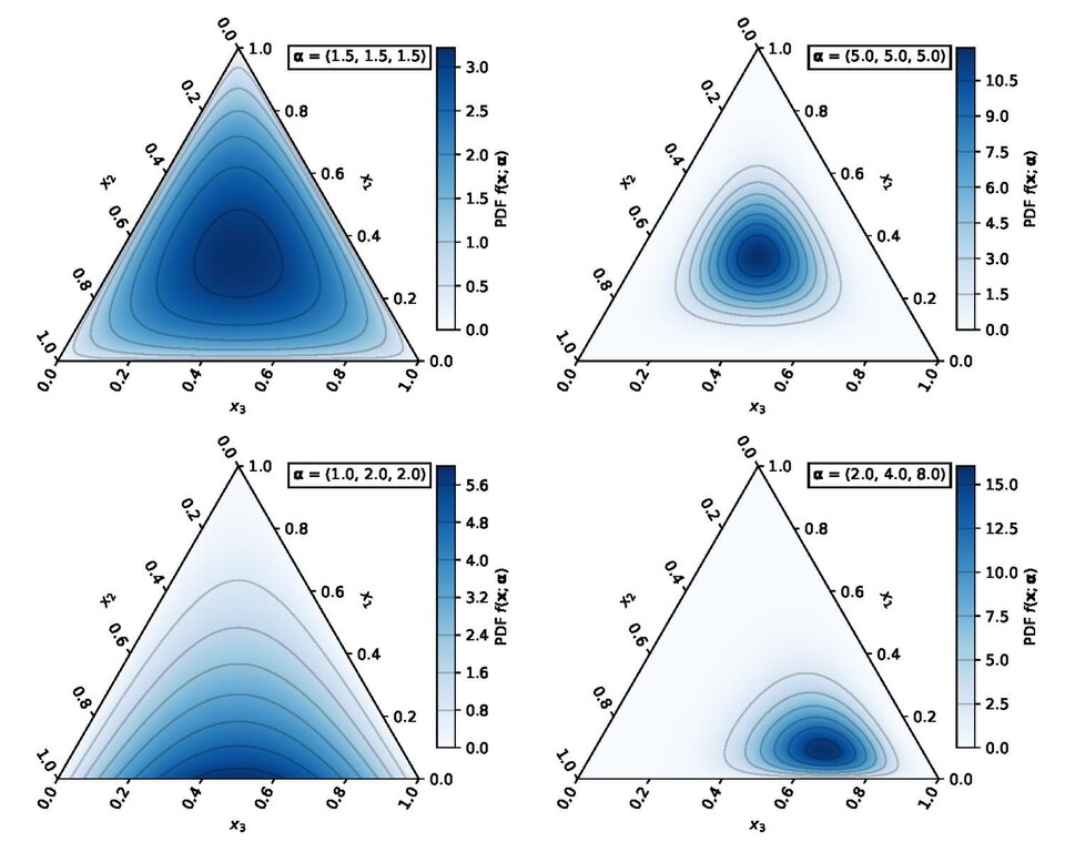
https://en.wikipedia.org/wiki/File:Dirichlet.pdf

Negative Binomial Softmax Regression

Why not transform proportions and run regression?

Transformation-based approaches are useful, but they may not fully account for:

zeros and low counts: log-ratios are undefined at zero and can be sensitive to pseudocounts;
finite sequencing depth: the same observed proportion can have very different precision across samples – transformation hides this;
heteroskedasticity: variability depends on abundance and sequencing depth;
feature-specific overdispersion: some features are inherently more variable than others;
the count-generating process: transformation separates the regression model from the mechanism that produced the observed counts.

Can we model counts directly while respecting compositional geometry?

The NBSR model

\[ y_{ij}\mid \pi_{ij},\phi_j \sim NB(n_i\pi_{ij},\phi_j), \]

\[ \pi_i=\operatorname{softmax}(\eta_i), \qquad \eta_{ij}=x_i^\top\beta_j. \]

NB likelihood

Probability distribution over counts, includes zero in the support.

Softmax mean

Fitted proportions $\pi_{ij}$ lie on the simplex.

Regression

Covariates explain compositional change.

How NBSR addresses the challenges

Challenge	NBSR component	How it helps
Zeros and low counts	Negative binomial likelihood	Models counts directly without requiring log transformation or pseudocounts
Finite sequencing depth	Mean structure ($n_i \pi_{ij}$)	Explicitly accounts for sample-specific sequencing depth
Heteroskedasticity	Negative binomial mean–variance relationship	Variance changes naturally with the expected count: $\text{Var}(Y_{ij}) = \mathbb{E}[Y_{ij}] + \phi_j \mathbb{E}[Y_{ij}]^2$
Feature-specific overdispersion	Feature-specific ($\phi_j$)	Allows different features to have different levels of extra-Poisson variation
Compositional constraint	Softmax link	Ensures $\pi_{ij}>0$ and $\sum_j \pi_{ij}=1$
Covariate effects	Regression on $\eta_{ij}=x_i^\top\beta_j$	Links predictors to changes in composition

Location, scale, and shape/dependence

Beyond differential abundance: location, scale, and shape/dependence

Many statistical models describe a distribution through three broad components:

Component	Scientific question	NBSR component
Location	How does the expected composition change?	Covariate effects ($\beta_j$)
Scale	How does residual variability change?	Dispersion ($\phi_j$)
Shape / dependence	How do features vary together across samples?	Latent factors ($z_i^\top\gamma_j$)

Most genomic analyses focus primarily on location: which features increase or decrease on average.

Our goal is to model not only the mean composition, but also changes in variability and shared dependence.

Why has statistical genomics focused on location?

The standard differential-expression question is:

Which genes/miRNAs/microbial taxa differ in average relative abundance?

This emphasis is understandable:

sample sizes are often modest;
location effects are easier to estimate and interpret;
power is limited for modeling higher-order distributional features;
many standard methods treat dispersion mainly as a nuisance parameter.

But disease may change more than the mean.

Location: changes in expected composition

For a binary condition $x_i\in \{0,1\}$,

\[ \eta_{ij} = \beta_{0j} + x_i\beta_{1j}, \qquad \pi_i=\operatorname{softmax}(\eta_i). \]

The coefficient $\beta_{1j}$ shifts the latent score of feature $j$ between conditions.

Through the softmax, all feature-specific shifts jointly determine the change in expected composition.

Because sequencing is relative, only contrasts among feature effects are identified from the observed counts.

More on how we will adjust the estimands later.

Why model scale?

Even within the same condition, biological samples do not have identical compositions.

For condition $g \in \{0,1\}$, suppose

\[ \pi_i \mid x_i=g \sim F\left(\boldsymbol{\lambda}^{(g)}\right), \]

where $\pi_i$ is the latent composition of sample $i$.

The observed count is then generated conditionally on that composition. For example,

\[ Y_{ij} \mid \pi_{ij},n_i \sim \operatorname{Poisson}(n_i\pi_{ij}). \]

Observed count variation therefore has two sources:

technical variability: repeated sequencing measurements of the same underlying composition would produce different finite-depth counts;
between-sample biological variability: the latent compositions $\pi_i$ differ across biological samples.

Coefficient of variation

Using the law of total variance,

\[ \operatorname{CV}^2(Y_{ij}) = \underbrace{\frac{1}{\mu_{ij}}}_{\text{Technical CV}^2} + \underbrace{\phi_j}_{\text{Biological CV}^2} \]

where $\mu_{ij} = n_i \mathbb{E}[\pi_{ij}]$ and $\phi_j$ is the squared coefficient of variation of the latent composition,

\[ \phi_j = \operatorname{CV}^2(\pi_{ij}) = \frac{\operatorname{Var}(\pi_{ij})}{\mathbb{E}[\pi_{ij}]^2}. \]

Thus, the dispersion parameter measures between-sample heterogeneity in the underlying composition, beyond finite sequencing noise.

A concrete example: the Dirichlet distribution

Suppose the latent composition follows

\[ \pi_i\mid x_i=g \sim \operatorname{Dirichlet} \left( \lambda_1^{(g)},\ldots,\lambda_K^{(g)} \right). \]

Let $\lambda_0^{(g)} = \sum_{k} \lambda_{k}^{(g)}$ and $\bar{\lambda}_j^{(g)} = \lambda_j^{(g)} / \lambda_0^{(g)}$. Then,

\[ \phi_j^{(g)} = \operatorname{CV}^2(\pi_{ij} \mid x_i=g) = \frac{ \left(1-\bar{\lambda}_j^{(g)}\right) }{ \bar{\lambda}_j^{(g)} (\lambda_0^{(g)}+1) }. \]

In general, for two conditions $g \neq g'$, biological variability may differ across conditions:

\[ \phi_j^{(g)} \neq \phi_j^{(g')}. \]

Modeling condition-dependent dispersion improves calibration

If dispersion differs across conditions but is modeled as constant, standard errors can be misestimated and confidence or credible intervals may be poorly calibrated.

This motivates modeling dispersion as a function of covariates:

\[ \log \phi_{ij} = w_{ij}^{\top} \alpha_j. \]

The scale covariates $w_{ij}$ may include,

disease or treatment group;
batch or other technical covariates;
functions of the expected proportion $\pi_{ij}$ or expected count $\mu_{ij}$.

Thus, variability may depend on both sample characteristics and the abundance level of the feature.

Note

The covariates governing variability need not be the same as those governing the mean composition.

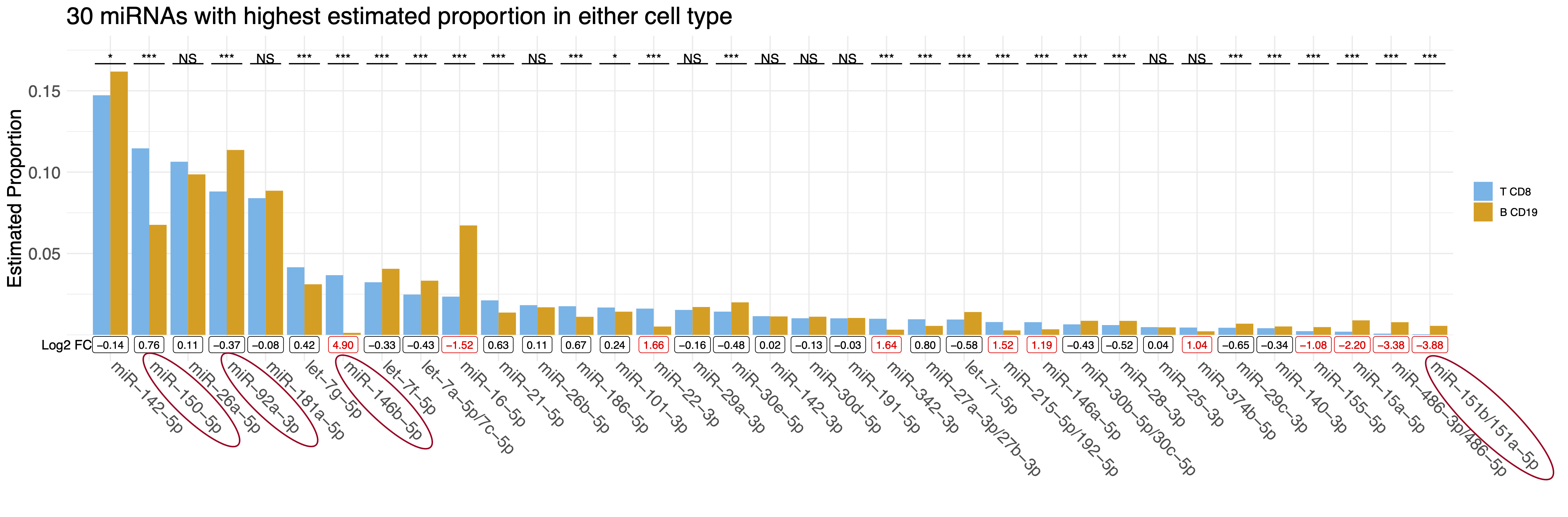
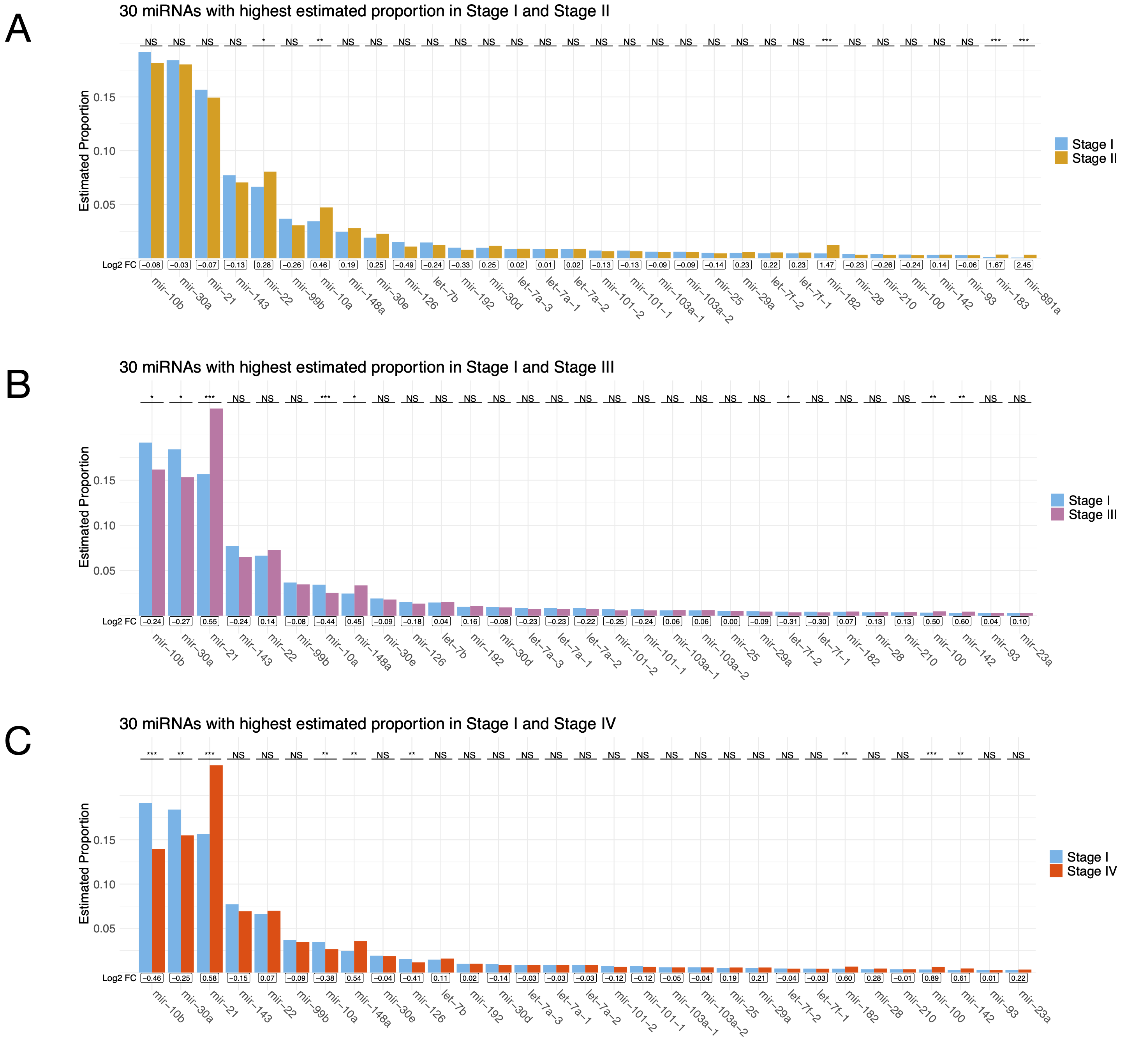
Real data provide justification for modeling scale

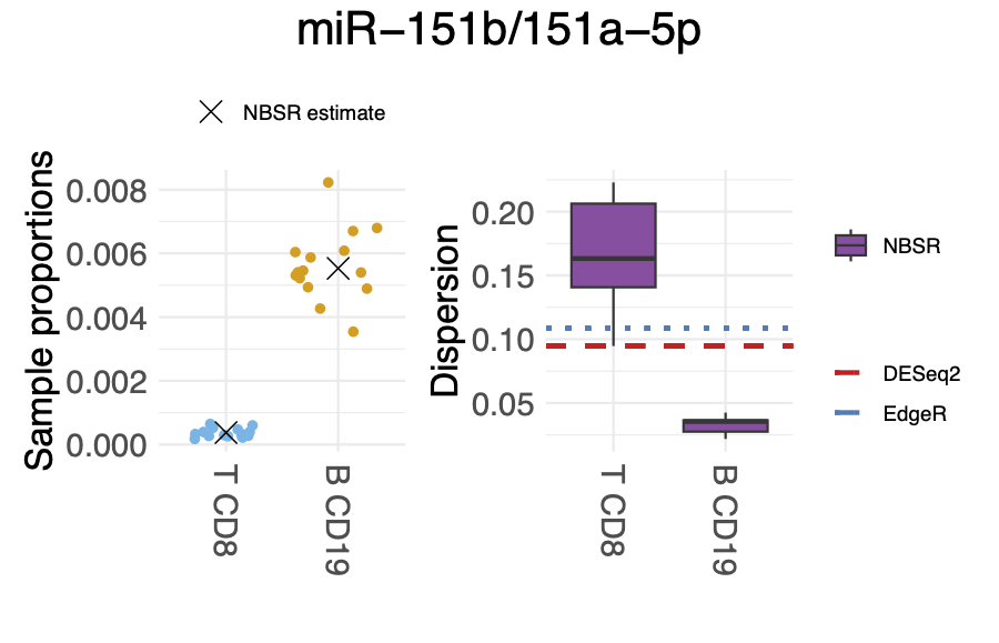
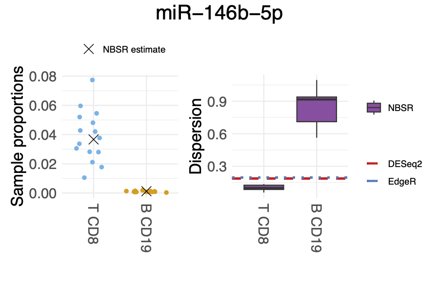
Location, scale, and shape

Location

How does the expected composition change?

\[ \beta_j \] Covariates shift the mean relative abundance of each feature.

Scale

How does biological heterogeneity change?

\[ \phi_j \]

Dispersion captures between-sample variability in the latent composition and may depend on covariates.

Shape / dependence

How do features co-vary beyond compositional constraints?

\[ z_i^\top\gamma_j \]

Latent factors capture shared residual structure across features.

Genomic studies have traditionally focused on location. Our framework extends this perspective by modeling scale, while ongoing work introduces latent factors to capture dependence and distributional shape.

Shape and dependence: latent factors

\[ \eta_{ij} = x_i^\top\beta_j + z_i^\top\gamma_j. \]

Latent factors can capture shared residual variation due to:

cell-type composition;
tumor purity;
immune infiltration;
batch or sequencing center;
sample quality;
unmeasured disease subtypes.

PhD student Xiangyi Chen is working on developing an efficient MCMC sampler for this problem.

Bayesian Inference

Posterior sampling

Let $\theta = (\beta, \alpha)$ denote all model parameters. The posterior distribution is,

\[ p(\theta \mid Y, X, W) = \frac{ p_{\ell}(Y | \theta, X, W) \cdot p_0(\theta). }{ m_0(Y | X, W) }. \]

The denominator $m_0$ denotes the marginal likelihood, which is intractable:

\[ m_0(Y | X, W) = \int p_{\ell}(Y | \theta, X, W) \cdot p_0(d\theta). \]

Two broad approaches are available:

Posterior sampling, such as Markov chain Monte Carlo (MCMC), provides full posterior inference but can be computationally expensive and requires convergence assessment.
Posterior approximation, such as the Laplace approximation, is usually much faster but relies on a local Gaussian approximation to the posterior.

Laplace approximation

The Laplace approximation replaces the posterior with a multivariate normal distribution centered at the posterior mode.

First optimize \[ \hat{\theta} = \operatorname{argmax}_{\theta} \log p(\theta | Y, X, W) \]

Evaluate Hessian of the log-posterior at $\hat{\theta}$, \[ H = \nabla_{\theta}^2 \log p(\theta | Y, X, W)\Big|_{\hat{\theta}} \]

Then, $\theta | Y, X, W \approx \operatorname{Normal}(\hat{\theta}, (-H)^{-1})$.

The approximation is most accurate when the posterior is unimodal and approximately symmetric near its mode.

Computing the Laplace approximation

The Laplace approximation requires two main steps:

Optimize the log-posterior to obtain the posterior mode $\hat{\theta}$;
Evaluate the Hessian at $\hat{\theta}$ to estimate the posterior covariance.

We use the automatic-differentiation framework PyTorch, which provides:

gradients for posterior optimization;
Hessian or Hessian-vector product calculations;
efficient implementation on CPUs or GPUs.

Inferential target

Recall, for feature $j$, our target is the absolute log-fold change:

\[ \delta_j = \log a_j^{(1)} - \log a_j^{(0)}. \]

But we can only estimate \[ \begin{aligned} d_j &= \log \pi_j^{(1)} - \log \pi_j^{(0)} \\ &= \delta_j - \Delta_{\text{total}}. \end{aligned} \]

Estimating the relative abundance effect

For $g \in \{0, 1\}$, let $x(g)$ denote the covariate vector corresponding to condition $g$. At the posterior mode,

\[ \hat{\pi}_{j}^{(g)} = \frac{ \exp(\hat{\beta}_j^\top x(g)) }{ \sum_{k} \exp(\hat{\beta}_k^{\top} x(g)) }. \]

So,

\[ \hat{d}_j = \log \hat{\pi}_j^{(1)} - \log \hat{\pi}_j^{(0)}. \]

We need to correct for the bias term: $\Delta_{\text{total}}$.

Bias correction

Suppose the absolute abundances under two conditions are

\[ (10, 10, 10, 10, 10) \quad \text{ and } \quad (20, 10, 10, 10, 10). \] Only the first feature changes. Therefore, the true absolute log-fold changes are

\[ \delta = (\log 2, 0, 0, 0, 0). \]

However, the corresponding compositions are

\[ \left(\frac{1}{5}, \frac{1}{5}, \frac{1}{5}, \frac{1}{5}, \frac{1}{5}\right) \quad \text{ and } \quad \left(\frac{2}{6}, \frac{1}{6}, \frac{1}{6}, \frac{1}{6}, \frac{1}{6}\right). \]

and the compositional log-fold change is

\[ d = \left(\log \frac{10}{6}, \log \frac{5}{6}, \log \frac{5}{6}, \log \frac{5}{6}, \log \frac{5}{6}\right). \]

All unchanged features are shifted by the same amount.

Bias correction: identifying the common shift

If most features are unchanged, then most $\delta_j$ values are zero:

\[ d_j = \delta_j - \Delta_{\text{total}} = - \Delta_{\text{total}} . \]

Therefore, the dominant mode of the $d_j$ values estimates,

\[ \hat{b} = -\hat{\Delta}_{\text{total}} = \text{mode} \{\hat{d}_1, ..., \hat{d}_K\}. \]

The bias corrected estimator is $\hat{\delta}_j = \hat{d}_j - \hat{b}$.

Note

The key assumption is that most features are unchanged, so the mode of the compositional effects represents the common compositional shift.

Real-data applications: Colon cancer cell lines

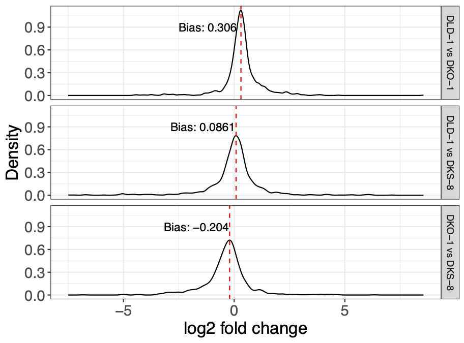
Delta-method inference

First, consider inference for the uncorrected compositional effect: $d_j = \log \pi_j^{(1)} - \log \pi_j^{(0)}$.

Under the Laplace approximation,

\[ \beta | Y, X, W \approx \operatorname{Normal}(\hat{\beta}, \Sigma_{\beta}), \] where $\Sigma_{\beta}$ is the block matrix of $(-H)^{-1}$ corresponding to $\beta$.

Using the delta method, we take $g_j(\beta) = d_j$:

\[ d_j \approx \operatorname{Normal}(\hat{d}_j, V_j), \] where $V_j = \nabla g_j(\hat{\beta})^{\top} \Sigma_{\beta} \nabla g_j(\hat{\beta})$.

Variance after bias correction

Recall that

\[ \hat{\delta}_j = \hat{d}_j - \hat{b}. \]

Therefore,

\[ \operatorname{Var}(\hat{\delta}_j) = \operatorname{Var}(\hat{d}_j) + \operatorname{Var}(\hat{b}) - 2 \operatorname{Cov}(\hat{d}_j, \hat{b}). \]

The latter two terms are difficult to derive analytically because $\hat{b}$ is the estimated mode of $\hat{d}_j$’s – a nonlinear function of all feature-level effects.

A simplified variance approximation

We use a computationally convenient approximation,

\[ \operatorname{Var}(\hat{\delta}_j) \approx \operatorname{Var}(\hat{d}_j). \]

Zhou et al. (2022) argue that, under suitable assumptions, these missing variance/covariance terms are small relative to the feature-specific variance.

We treat this as a working approximation and assess its adequacy empirically.

Simulations and data analysis

Simulation goals

We evaluate whether the proposed method provides:

false-discovery-rate control and adequate power;
accurate effect and dispersion estimation;
calibrated interval estimates;
robustness to compositional shifts;
adaptation to feature- and condition-specific dispersion.

We compare NBSR with DESeq2, edgeR, and LinDA.

Simulated data generating framework

We simulate counts in two conditions, $g \in \{0,1\}$.

For sample $i$ in condition $g$:

Sample a composition:

\[ \pi_i \sim \text{Dirichlet}(\lambda^{(g)}). \] 2. Sample the total number of reads, $s_i = \lceil u_i \rho_i \rceil$ where $u_i \sim \operatorname{Uniform}(10^6, 10^8)$ models the library size and $\rho_i ~ \text{Uniform}(0, 0.5)$ models the capture rate for miRNA molecules.

Generate sequencing counts \[ Y_i \sim \text{Multinomial}(s_i \pi_i). \]

Real data calibration

The baseline Dirichlet parameters $\lambda$ are estimated from real microRNAome datasets [McCall et al (2017)].

We retain human miRNAs listed in MirGeneDB [Fromm et al (2022)]; samples with fewer than $100{,}000$ miRNA reads are excluded; the final analysis includes $K=596$ miRNAs.

Dirichlet parameters are estimated separately for each cell type.

This produces realistic differences in:

baseline abundance;
feature-specific variability;
compositional competition;
sparsity and dynamic range.

Simulating changes in abundances

Randomly select indices $\mathcal{I} \in \{1, ..., K\}$;
Sample $f_j > 0$ for $j \in \mathcal{I}$;
$\lambda_j^{(1)} = f_j \lambda_j^{(0)}$.

Categorize features into {HIGH, MED, LOW} based on $\lambda_j^{(0)}$.
Bound the fold change values $f_j$; e.g., if $\lambda_j^{(0)}$ is highly abundant, it does not make sense for it to be increased twofold.

Simulation results 1: FDR and power

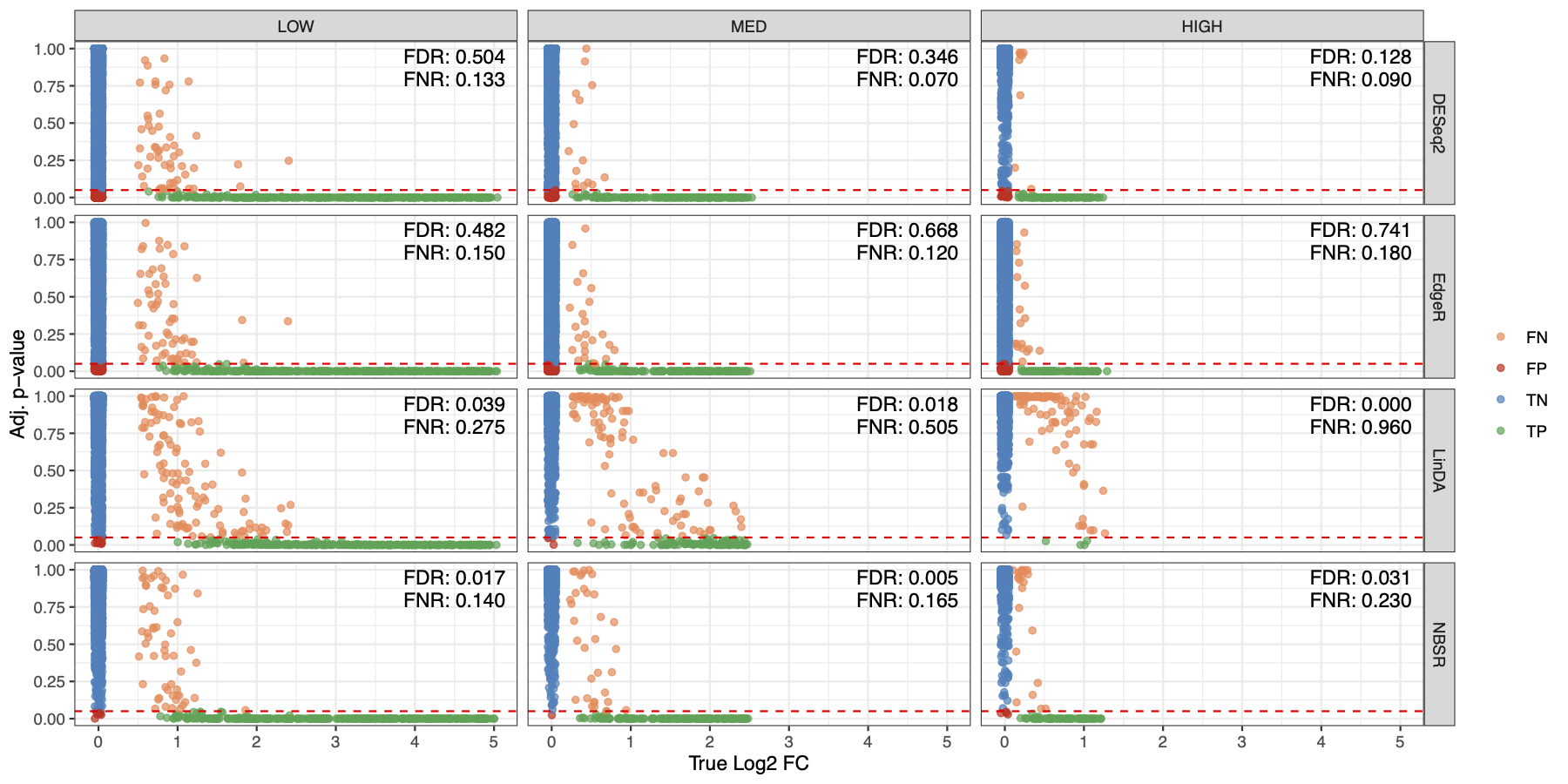
NBSR controls false discoveries across abundance levels.

Simulation results 2: heterogeneity in dispersion

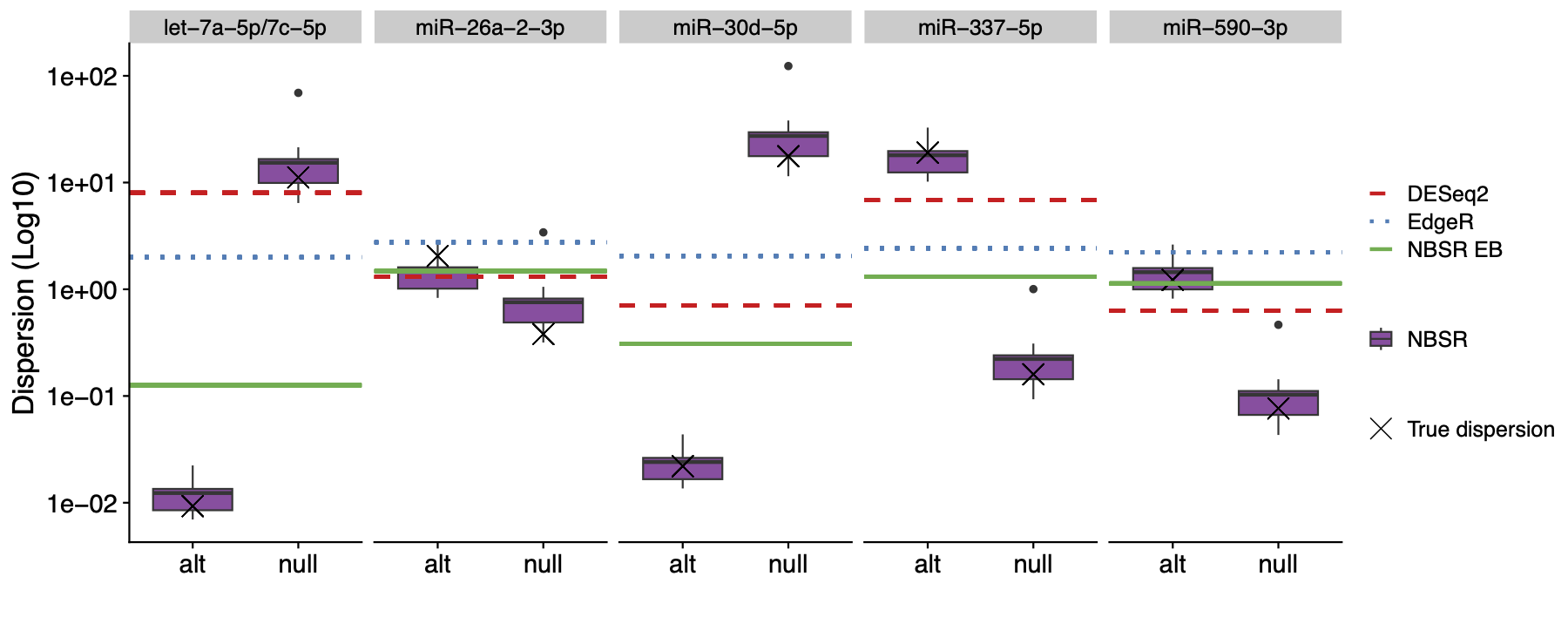
NBSR provides accurate estimates for the dispersion parameter.

Simulation results 3: effect estimation

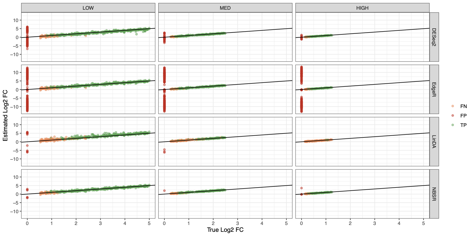
Bias correction recovers feature-specific effects.

Simulation results 4: coverage

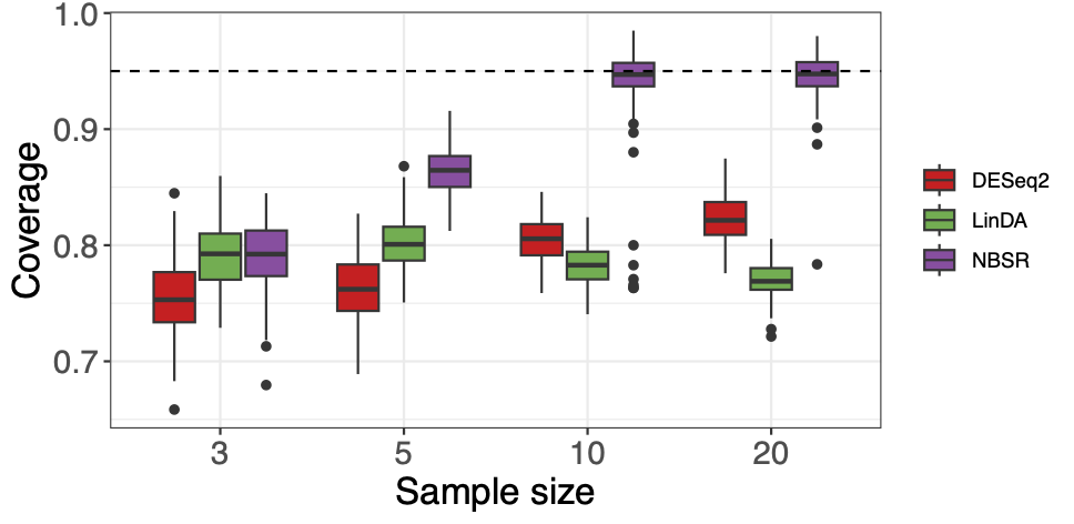
Modeling condition-dependent dispersion maintains coverage near the nominal level when biological variability differs across groups.

Weaknesses of Laplace approximation

The Laplace approximation provides fast inference and good false-discovery-rate control.

However, it can be conservative:

credible intervals may be wider than those obtained from full posterior sampling;
true differential features may therefore be missed;
this leads to a higher false-negative rate and reduced power.

How much efficiency do we lose by replacing full posterior sampling with a local Gaussian approximation?

Approximate versus sampling-based inference

The fast Laplace approach uses a delta-method approximation for the relative effect,

\[ d_j = \log\pi_j^{(1)} - \log\pi_j^{(0)}. \]

After estimating the common compositional shift (b),

\[ \hat\delta_j=\hat d_j-\hat b. \]

The exact variance contains additional terms:

\[ \operatorname{Var}(\hat\delta_j) = \operatorname{Var}(\hat d_j) + \operatorname{Var}(\hat b) - 2\operatorname{Cov}(\hat d_j,\hat b). \]

For computational convenience, our current Laplace procedure uses

\[ \operatorname{Var}(\hat\delta_j) \approx \operatorname{Var}(\hat d_j), \]

and therefore does not fully propagate uncertainty from estimating the common shift.

Full posterior sampling produces narrower intervals

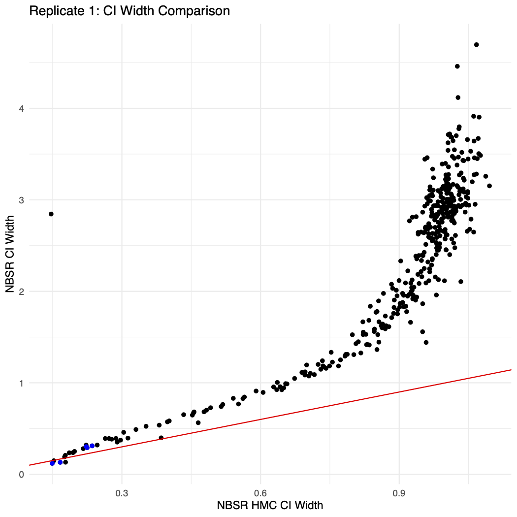
Each point represents one feature. Credible interval width from HMC (x-axis) and for Laplace approximation (y-axis).

Most points lie above the diagonal, indicating that the Laplace approximation produces wider credible intervals than HMC.

Full posterior sampling produces narrower intervals

For each posterior draw $s$, HMC recomputes the common shift $b$ and the corrected effect

\[ \delta_j^{(s)}=d_j^{(s)}-b^{(s)}. \]

It therefore propagates the uncertainty in $b$ and its dependence with $d_j$, rather than dropping these terms.

Open problems

This area has many open methodological questions:

scalable Bayesian computation;
longitudinal and spatial compositions;
single-cell RNA-seq data;
multimodal integration;
causal interpretation of differential abundance.

Opportunities for students

This project sits at the intersection of:

Bayesian modeling
compositional data analysis
high-dimensional statistics
scientific computing

computational biology
cancer genomics
microbiome research
software development

Students can contribute to new theory, computation, software, and biomedical applications.

PhD Opportunities at the University of Rochester

PhD in Statistics

Department of Biostatistics and Computational Biology

rigorous training in statistical theory and methodology
close faculty mentorship in a small, collaborative program
direct collaboration with biomedical and health-science researchers
opportunities in statistical genomics, computational biology, and data science
optional concentration in Bioinformatics and Computational Biology

The program is housed within the School of Medicine and Dentistry, connecting methodological research directly to substantive scientific problems.

Where our graduates go

Graduates pursue careers in:

universities and academic medical centers;
pharmaceutical and biotechnology companies;
government and public-health organizations;
healthcare and biomedical research institutions.

Link

Funding and program structure

All admitted Statistics PhD students receive:

full tuition support
individual health-insurance coverage
a 10-month stipend of $29,250 for 2026–2027
- opportunities for summer support or external internships
funding regardless of citizenship status

Years 1–2: Funding is provided by the School of Medicine and Dentistry.

Year 3 onward: The department supports students through collaborative biomedical research, training grants, and methodological research grants.

Students are matched with projects based on mutual research interests and are not required to secure their own academic-year funding.

The program generally takes 4–6 years, with most students completing the degree in five years. Up to 30 graduate credits may be transferred, subject to approval.

Applying to the Statistics PhD program

Important dates

November 15, 2026: Submit by this date for an automatic application-fee waiver
December 1, 2026: Priority application deadline
December 15, 2026: Final Statistics PhD application deadline

What the Admissions Committee values

mathematical/statistical preparation
letters of recommendation
statement of purpose
research experience, when available

The GRE is not considered, even if submitted.

Most international applicants must submit TOEFL, IELTS, or Duolingo scores. Waivers are available in specified circumstances.

Thank you

Questions?

Seong-Hwan Jun
Email: seonghwan_jun@urmc.rochester.edu

Bibliography

van Nood, E. et al. Duodenal infusion of donor feces for recurrent Clostridium difficile. N. Engl. J. Med. 368, 407–415 (2013).

Zhou, H., He, K., Chen, J. & Zhang, X. LinDA: linear models for differential abundance analysis of microbiome compositional data. Genome Biol. 23, 95 (2022).

McCall, M. N. et al. Toward the human cellular microRNAome. Genome Res. 27, 1769–1781 (2017).

Fromm, B. et al. MirGeneDB 2.1: toward a complete sampling of all major animal phyla. Nucleic Acids Res. 50, D204–D210 (2022).

Backup slides

Backup: negative binomial parameterization

\[ y_{ij}\mid \pi_{ij},\phi_j\sim \operatorname{NB}(n_i\pi_{ij},\phi_j), \]

\[ E(y_{ij})=\mu_{ij}, \qquad \operatorname{Var}(y_{ij})=\mu_{ij}+\phi_j\mu_{ij}^2. \]

Ratios are natural quantities

A basic log-ratio is

\[ \log \frac{\pi_j}{\pi_k}. \]

Interpretation:

How abundant is feature $j$ relative to feature $k$?

Log-ratios turn multiplicative comparisons into additive quantities suitable for regression.

ALR, CLR, and ILR at a glance

ALR

\[ \log\frac{\pi_j}{\pi_K} \]

Uses a reference feature.

CLR

\[ \log\frac{\pi_j}{g(\pi)} \]

Uses the geometric mean.

ILR

Orthonormal log-contrast coordinates.

ALR, CLR, and ILR at a glance

Transformation	Definition	Advantages	Limitations
ALR	$\displaystyle \log\frac{\pi_j}{\pi_K}$	Easy to compute and fit using standard regression methods; directly interpretable relative to a chosen reference $K$	Results depend on the reference; an unstable or changing reference affects every coordinate
CLR	$\displaystyle \log\frac{\pi_j}{g(\pi)}$	Symmetric across features; does not require a single reference feature	Coordinates sum to zero; covariance matrix is singular; interpretation is relative to the geometric mean
ILR	$\displaystyle z = V^\top \log \pi$	Orthonormal and nonredundant; well suited for standard multivariate methods	Coordinates depend on the chosen basis; often less directly interpretable biologically

Backup: CLR definition

For $\pi\in S^K$, define

\[ CLR(\pi)_j = \log\frac{\pi_j}{g(\pi)}, \qquad g(\pi)=\left(\prod_{k=1}^K \pi_k\right)^{1/K}. \]

Backup: softmax and inverse CLR

\[ \operatorname{softmax}(\eta)_j = \frac{\exp(\eta_j)}{\sum_k\exp(\eta_k)}. \]

Let $\tilde\eta=\eta-\bar\eta\mathbf{1}$. Then

\[ \operatorname{softmax}(\eta)=CLR^{-1}(\tilde\eta). \]

Backup: ALR-to-CLR centering

Under an ALR reference constraint, $\beta_K=0$. The reference-free CLR coefficient is

\[ \beta_j^{CLR} = \beta_j^{ALR} - \frac{1}{K}\sum_{k=1}^K\beta_k^{ALR}. \]

Backup: direct CLR contrast

For a binary condition without interactions,

\[ \Delta_j^{CLR} = \beta_j - \frac{1}{K}\sum_{k=1}^K\beta_k. \]

This is invariant to the ALR reference.

Posterior bias correction

For each posterior draw $s$:

calculate $\Delta_j^{CLR,(s)}$;
estimate the global center $m_b^{(s)}$;
compute

\[ \Delta_j^{adj,(s)} = \Delta_j^{CLR,(s)}-m_b^{(s)}; \]

summarize across posterior draws.

Note

The uncertainty in the bias correction is propagated automatically.

Simulation scenarios

Two cases:

Total abundance conserved. Swap parameters between low- and high-abundance features; increases are balanced by corresponding decreases; considers sample sizes $N \in \{3, 5, 10, 20\}$ per group.
Total abundance imbalanced.

Multiply selected parameters by randomly sampled fold change values;
Perturb $5, 10, 20$ features from high, medium, and low abundance groups;
Sample sizes $N \in \{3, 5, 10\}$ per group.

Component	Scientific question	NBSR component
Location	How does the expected composition change?	Covariate effects (\(\beta_j\))
Scale	How does residual variability change?	Dispersion (\(\phi_j\))
Shape / dependence	How do features vary together across samples?	Latent factors (\(z_i^\top\gamma_j\))

Transformation	Definition	Advantages	Limitations
ALR	\(\displaystyle \log\frac{\pi_j}{\pi_K}\)	Easy to compute and fit using standard regression methods; directly interpretable relative to a chosen reference \(K\)	Results depend on the reference; an unstable or changing reference affects every coordinate
CLR	\(\displaystyle \log\frac{\pi_j}{g(\pi)}\)	Symmetric across features; does not require a single reference feature	Coordinates sum to zero; covariance matrix is singular; interpretation is relative to the geometric mean
ILR	\(\displaystyle z = V^\top \log \pi\)	Orthonormal and nonredundant; well suited for standard multivariate methods	Coordinates depend on the chosen basis; often less directly interpretable biologically