class: ur-title, center, middle, title-slide .title[ # BST430 Lecture 05 ] .subtitle[ ## Data transformation with dplyr ] .author[ ### Seong-Hwan Jun, based on the course by Andrew McDavid ] .institute[ ### U of Rochester ] .date[ ### 2021-08-31 (updated: 2025-09-09 by TL) ] --- ## Announcements - HW1 assigned, due next Wednesday 5pm. - Reminder: lab 2 due at 5pm. - TA office hours are posted on class website. + Hanwen: Thursday 1 - 2 pm. + Abby: 12:15 - 1:15 pm. - I don't have office hour but email me if you need to talk to me. --- # Agenda - The pipe - Manipulating data frames. - Calculating summary statistics. - Using the basic functions of `dplyr` - grouping by multiple variables - empty groups and summarizing - ungrouping - grouped mutates and filters - special selection operators - repeating operations on multiple columns with `across` --- class: center, middle # Pipes --- ## Where does the name come from? We have already seen the `%>%` operator a bit. The pipe operator is implemented in the package **magrittr**. <!-- <sup>1</sup> --> .pull-left[  ] .pull-right[  ] <!-- .footnote[[1] In R 4.1, there is also support for a variant of the pipe with `|>`. It behaves similarly, but not identically to magrittr's `%>%`. For the moment, personally, I am holding off using it in this course or in my own projects to avoid a hard dependency on R 4.1.] --> <!-- ??? --> <font size="3"> "The Treachery of Images" is a 1929 painting by Belgian surrealist painter René Magritte. <!-- It is also known as This Is Not a Pipe[2]. It is on display at the Los Angeles County Museum of Art.[1] --> The painting shows an image of a pipe. Below it, Magritte painted, "Ceci n'est pas une pipe", French for "This is not a pipe". </font> > The famous pipe. How people reproached me for it! And yet, could you stuff my pipe? No, it's just a representation, is it not? So if I had written on my picture "This is a pipe", I'd have been lying! --- ## How does a pipe work? - You can think about the following sequence of actions - find your helmet, ride your bike to school, then lock it somewhere. - Expressed as a set of nested functions in R pseudocode this would look like: ```r lock(ride(find(who=tanzy, what = "helmet"), to = "campus")) ``` we have to read this from the "inside-out". --- ## How does a pipe work? - The pipe gives it a more natural (and easier to read) **postfix** syntax<sup>1</sup>, where we can read from left to right: ```r tanzy %>% find(what = "helmet") %>% ride(to = "campus") %>% lock() ``` .footnote[[1] Note similar syntax in java(script), C++ and python where the method accessor "`.`" can be chained in some cases: `tanzy.find('helmet').ride('campus').lock()`] --- ## What about other arguments? The pipe, by default sends its left-hand value to first positional argument of the right-hand function. To send results to a function argument other than first one or to use the previous result for multiple arguments, use `.`: ```r starwars %>% filter(species == "Human") %>% lm(mass ~ height, data = .) ``` ``` ## ## Call: ## lm(formula = mass ~ height, data = .) ## ## Coefficients: ## (Intercept) height ## -81.7726 0.9048 ``` --- ## Useful tips - Shortcut for piping: cmd/ctrl + shift + M. - Since R 4.1, there is also a native pipe operator `|>` in base R. Enable this `Tools-> Global Options -> Code -> Use R native pipe operator`. - It is always available even when you are not using `tidyverse`. --- ## Useful tips - `|>` behaves similarly, but not identically to magrittr's `%>%`. + To send results to a function argument other than first one or to use the previous result for multiple arguments, use `_` instead of `.`. ```r starwars |> lm(mass ~ height, data = _) ``` ``` ## ## Call: ## lm(formula = mass ~ height, data = starwars) ## ## Coefficients: ## (Intercept) height ## -11.487 0.624 ``` <!-- --- --> <!-- ## The pipe vs ggplot2 layers --> <!-- - The `+` operator in **ggplot2**<sup>1</sup> is used for "layering." This means you create the plot in layers, separated by `+`. --> <!-- - Some of the reason for this distinction is historical rather than mechanistic --> <!-- .footnote[[1] to make matters even more confusing, ggplot2 also has the `%+%` operator. This modifies the `data` being used in the plot.] --> --- class: center, middle # Data transformation --- ## NYC Flights ```r library(nycflights13) ``` This data frame contains all 336,776 flights that departed from New York City in 2013. The data comes from the US [Bureau of Transportation Statistics](http://www.transtats.bts.gov/DatabaseInfo.asp?DB_ID=120&Link=0), and is documented in `?flights`. --- # Want to follow along? Here's the [R code in this lecture](https://github.com/seonghwanjun/bst430-fall2025-l05/blob/main/transform-dplyr-i.R) <!-- Go to RStudio Cloud and make a copy of "Lecture 3 - dplyr" --> --- ## Viewing your data - In the Environment, click on the name of the data frame to view it in the data viewer - Use the `glimpse` function to take a peek .scroll-box-14[ ```r glimpse(flights) ``` ``` ## Rows: 336,776 ## Columns: 19 ## $ year <int> 2013, 2013, 2013, 2013, 2013, 2013,… ## $ month <int> 1, 1, 1, 1, 1, 1, 1, 1, 1, 1, 1, 1,… ## $ day <int> 1, 1, 1, 1, 1, 1, 1, 1, 1, 1, 1, 1,… ## $ dep_time <int> 517, 533, 542, 544, 554, 554, 555, … ## $ sched_dep_time <int> 515, 529, 540, 545, 600, 558, 600, … ## $ dep_delay <dbl> 2, 4, 2, -1, -6, -4, -5, -3, -3, -2… ## $ arr_time <int> 830, 850, 923, 1004, 812, 740, 913,… ## $ sched_arr_time <int> 819, 830, 850, 1022, 837, 728, 854,… ## $ arr_delay <dbl> 11, 20, 33, -18, -25, 12, 19, -14, … ## $ carrier <chr> "UA", "UA", "AA", "B6", "DL", "UA",… ## $ flight <int> 1545, 1714, 1141, 725, 461, 1696, 5… ## $ tailnum <chr> "N14228", "N24211", "N619AA", "N804… ## $ origin <chr> "EWR", "LGA", "JFK", "JFK", "LGA", … ## $ dest <chr> "IAH", "IAH", "MIA", "BQN", "ATL", … ## $ air_time <dbl> 227, 227, 160, 183, 116, 150, 158, … ## $ distance <dbl> 1400, 1416, 1089, 1576, 762, 719, 1… ## $ hour <dbl> 5, 5, 5, 5, 6, 5, 6, 6, 6, 6, 6, 6,… ## $ minute <dbl> 15, 29, 40, 45, 0, 58, 0, 0, 0, 0, … ## $ time_hour <dttm> 2013-01-01 05:00:00, 2013-01-01 05… ``` ] --- class: font120 ## A Grammar of Data Manipulation **dplyr** is based on the concepts of functions as verbs that manipulate data frames. Single data frame functions / verbs: <!-- <font size = "3"> --> * `filter`: pick rows matching criteria * `slice`: pick rows using index(es) * `select`: pick columns by name * `pull`: grab a column as a vector * `rename`: rename specific columns * `arrange`: reorder rows * `mutate`: add new variables * <s>`transmute`: create new data frame with variables</s> superseded by `mutate(.keep="none")` * `distinct`: filter for unique rows * <s>`sample_n` / `sample_frac`: randomly sample rows</s> superseded by `slice_sample()` * `summarise`: reduce variables to values * `group_by`: run an operation by levels of a categorical variable * ... (many more) <!-- </font> --> --- ## **dplyr** rules for functions 1. First argument is *always* a `data.frame`<sup>1</sup> 2. Subsequent arguments say what to do with that `data.frame` 3. Always return a new `data.frame` 4. Doesn't modify in place .footnote[[1] Or `tibble`, the tidyverse version of a `data.frame`.] --- ## Filter rows with `filter` - Select a subset of rows in a data frame based on when a logical expression returns `TRUE` - Easily filter for many conditions at once by combining logical expressions *remember* we used filter in lab 1 ``` dino_data = datasaurus_dozen %>% filter(dataset == "dino") ``` --- class: code70 ## `filter` - Let's extract all flights from new york that occurred in April. ```r flights %>% filter(month == 4) ``` ``` ## # A tibble: 28,330 × 19 ## year month day dep_time sched_dep_time dep_delay ## <int> <int> <int> <int> <int> <dbl> ## 1 2013 4 1 454 500 -6 ## 2 2013 4 1 509 515 -6 ## 3 2013 4 1 526 530 -4 ## 4 2013 4 1 534 540 -6 ## # ℹ 28,326 more rows ## # ℹ 13 more variables: arr_time <int>, ## # sched_arr_time <int>, arr_delay <dbl>, carrier <chr>, … ``` --- class: code70 ## `filter` with multple conditions - You can filter based on more than two variables using logical operators. - All flights that were both in April and from JFK: ```r flights %>% filter(month == 4 & origin == "JFK") ``` ``` ## # A tibble: 9,218 × 19 ## year month day dep_time sched_dep_time dep_delay ## <int> <int> <int> <int> <int> <dbl> ## 1 2013 4 1 534 540 -6 ## 2 2013 4 1 542 545 -3 ## 3 2013 4 1 543 545 -2 ## 4 2013 4 1 555 600 -5 ## # ℹ 9,214 more rows ## # ℹ 13 more variables: arr_time <int>, ## # sched_arr_time <int>, arr_delay <dbl>, carrier <chr>, … ``` --- class: code70 ## `filter` with multple conditions - `filter()` will also perform the **and** operation if you separate logical conditions by a comma. ```r flights %>% filter(month == 4, origin == "JFK") ``` ``` ## # A tibble: 9,218 × 19 ## year month day dep_time sched_dep_time dep_delay ## <int> <int> <int> <int> <int> <dbl> ## 1 2013 4 1 534 540 -6 ## 2 2013 4 1 542 545 -3 ## 3 2013 4 1 543 545 -2 ## 4 2013 4 1 555 600 -5 ## # ℹ 9,214 more rows ## # ℹ 13 more variables: arr_time <int>, ## # sched_arr_time <int>, arr_delay <dbl>, carrier <chr>, … ``` --- ## Aside: enumerating a categorical variable - If you didn't know what origins were possible in the `flights` data, then you can take one of two approaches: 1. `unique()` 2. `table(x, exclude = NULL)` to get the counts of each level. The `exclude = NULL` indicates that `NA` missing values should also be listed -- you almost certainly want this! ```r unique(flights$origin) ``` ``` ## [1] "EWR" "LGA" "JFK" ``` ```r table(flights$origin, exclude = NULL) ``` ``` ## ## EWR JFK LGA ## 120835 111279 104662 ``` --- ## Boolean expressions - This code finds all flights that departed in November or December: ```r filter(flights, month == 11 | month == 12) ``` The order of operations doesn't work like English. You can't write `filter(flights, month == (11 | 12))`, to mean "find all flights that departed in November or December." - Instead, this would find all months that equal `11 | 12`, an expression that evaluates to `TRUE`. - In a numeric context (like here), `TRUE` is coerced to `1`, so this finds all flights in January, not November or December. This *is* quite confusing! --- ## Boolean expressions But this works: ```r filter(flights, month %in% c(11,12)) ``` ``` ## # A tibble: 55,403 × 19 ## year month day dep_time sched_dep_time dep_delay ## <int> <int> <int> <int> <int> <dbl> ## 1 2013 11 1 5 2359 6 ## 2 2013 11 1 35 2250 105 ## 3 2013 11 1 455 500 -5 ## 4 2013 11 1 539 545 -6 ## # ℹ 55,399 more rows ## # ℹ 13 more variables: arr_time <int>, ## # sched_arr_time <int>, arr_delay <dbl>, carrier <chr>, … ``` Saves a bit of typing. --- class: code70, font120 ## Missing Values - `filter()` .alert[excludes] observations with .alert[missing values.] ```r dfdat = tibble(x = c(1, 2, NA), y = c('A', 'B', 'C')) dfdat ``` ``` ## # A tibble: 3 × 2 ## x y ## <dbl> <chr> ## 1 1 A ## 2 2 B ## 3 NA C ``` ```r dfdat %>% filter(x == 1) ``` ``` ## # A tibble: 1 × 2 ## x y ## <dbl> <chr> ## 1 1 A ``` - If you want to extract those rows as well, you have to ask for them explicitly using `is.na()`: ```r dfdat %>% filter(x == 1 | is.na(x)) ``` ``` ## # A tibble: 2 × 2 ## x y ## <dbl> <chr> ## 1 1 A ## 2 NA C ``` --- class: code70 ## Missing Values are contagious ```r NA > 5; 10 == NA; NA + 10 ``` ``` ## [1] NA ``` ``` ## [1] NA ``` ``` ## [1] NA ``` - Therefore, **you cannot test for missingness with `== NA`**: ```r x = NA x == NA ``` ``` ## [1] NA ``` ```r is.na(x) ``` ``` ## [1] TRUE ``` --- ## Graphical Depiction of Logical Operations: <!-- --> --- ## Commonly used logical operators in R operator | definition || operator | definition ------------ | ------------------------------ || -------------- | ---------------- `<` | less than ||`x` | `y` | `x` OR `y` `<=` | less than or equal to ||`is.na(x)` | test if `x` is `NA` `>` | greater than ||`!is.na(x)` | test if `x` is not `NA` `>=` | greater than or equal to ||`x %in% y` | test if `x` is in `y` `==` | exactly equal to ||`!(x %in% y)` | test if `x` is not in `y` `!=` | not equal to ||`!x` | not `x` `x & y` | `x` AND `y` || | --- ## Check your understanding Using the `flights` data frame from the `nycflights13` package, write code to do the following tasks: 1. .question[Extract the January LGA flights and the December JFK flights.] 2. .question[Extract flights whose `dep_time` was `NA`.] 3. .question[Extract flights that left in odd months (i.e., 1, 3, 5, 7, 9, 11).] --- ## Answers ``` flights %>% filter((month == 1 & origin == "LGA") | (month == 12 & origin == "JFK")) ``` ``` flights %>% filter(is.na(dep_time)) ``` ``` flights %>% filter(month %in% seq(1, 11, 2)) ``` --- ## Create New Variables - The variables given are usually not enough for an analysis. - For instance: + log-transform positive values to make associations more linear. + recode categorical variables to add / remove levels + clean up messy text data + ... or any other mathematical or CS .alert[vector function] of the data. --- class: code70 ## `mutate` to add new variables - We can use `mutate()` to create new variables from old. ```r temp=flights %>% mutate(gain = dep_delay - arr_delay, speed = distance / air_time * 60, .before = year) #add before `year` variable colnames(temp) ``` ``` ## [1] "gain" "speed" "year" "month" ## [5] "day" "dep_time" "sched_dep_time" "dep_delay" ## [9] "arr_time" "sched_arr_time" "arr_delay" "carrier" ## [13] "flight" "tailnum" "origin" "dest" ## [17] "air_time" "distance" "hour" "minute" ## [21] "time_hour" ``` --- class: code70 ## `mutate` to add new variables ```r temp[,c("gain","speed")] ``` ``` ## # A tibble: 336,776 × 2 ## gain speed ## <dbl> <dbl> ## 1 -9 370. ## 2 -16 374. ## 3 -31 408. ## 4 17 517. ## # ℹ 336,772 more rows ``` --- ## Converting to minutes since midnight - **Exercise**: `dep_time` is convenient to look at, but hard to compute with because it's not a continuous value: ```r ggplot(flights, aes(x = dep_time)) + geom_histogram(binwidth = 10) ``` <!-- --> --- ## Check your understanding - Convert `dep_time` into `dep_minutes_midnight`, the number of minutes since midnight. Hint: `%/%` is truncating integer division and `%%` is remainder. For instance: ```r 101 / 10 ``` ``` ## [1] 10.1 ``` ```r 101 %/% 10 ``` ``` ## [1] 10 ``` ```r 101 %% 10 ``` ``` ## [1] 1 ``` --- ## Answer ```r flights %>% mutate(dep_h = dep_time %/% 100, dep_m = dep_time %% 100, dep_elapsed_min = dep_h * 60 + dep_m, .after=dep_time) ``` ``` ## # A tibble: 336,776 × 22 ## year month day dep_time dep_h dep_m dep_elapsed_min ## <int> <int> <int> <int> <dbl> <dbl> <dbl> ## 1 2013 1 1 517 5 17 317 ## 2 2013 1 1 533 5 33 333 ## 3 2013 1 1 542 5 42 342 ## 4 2013 1 1 544 5 44 344 ## # ℹ 336,772 more rows ## # ℹ 15 more variables: sched_dep_time <int>, ## # dep_delay <dbl>, arr_time <int>, … ``` --- ## Only preserving new variables If you only want to keep new variables, use `transmute()` ```r flights %>% transmute(gain = dep_delay - arr_delay, hours = air_time / 60, gain_per_hour = gain / hours) ``` ``` ## # A tibble: 336,776 × 3 ## gain hours gain_per_hour ## <dbl> <dbl> <dbl> ## 1 -9 3.78 -2.38 ## 2 -16 3.78 -4.23 ## 3 -31 2.67 -11.6 ## 4 17 3.05 5.57 ## # ℹ 336,772 more rows ``` This function has been superseded now by `mutate(.keep="none")`. --- ## Only preserving new variables ```r flights %>% mutate(gain = dep_delay - arr_delay, hours = air_time / 60, gain_per_hour = gain / hours, .keep = "none") ``` ``` ## # A tibble: 336,776 × 3 ## gain hours gain_per_hour ## <dbl> <dbl> <dbl> ## 1 -9 3.78 -2.38 ## 2 -16 3.78 -4.23 ## 3 -31 2.67 -11.6 ## 4 17 3.05 5.57 ## # ℹ 336,772 more rows ``` --- ## Useful mutation functions - Arithmetic operators: `+`, `-`, `*`, `/`, `^` - Arithmetic operators in conjunction with scalar functions: + `x_center = x - mean(x)` + `x_proportion = x / sum(x)` + `x_01 = (x-min(x))/(max(x) - min(x))` - Modular arithmetic: `%/%` (integer division) and `%%` (remainder) - Logs: `log()`, `log2()`, `log10()` - offsets: `lead()` and `lag()` - Cumulative and rolling aggregates: `cumsum()`, `cumprod()`, `cummin()`, `cummax()`, `cummean()`. - Ranking: `min_rank()`. Mind how `NA` and ties are handled! - Recoding: `case_when()`, `ifelse()` --- ## Recoding with `case_when` and `ifelse` - `case_when` lets us generate a new variable with multiple values that depend on arbitrary boolean expressions. - Each boolean expression is evaluated in turn, and the first matching value is used. - The syntax is ```r case_when(<BOOLEAN EXPRESSION 1> ~ "value1", <BOOLEAN EXPRESSION 2> ~ "value2", <more expressions and values>, TRUE ~ "Optional fallthrough value") ``` - If the `TRUE ~ "Optional fallthrough"` isn't provided and no cases match, than the value will be `NA`. - `ifelse` is a simplified version: ```r ifelse(<BOOLEAN EXPRESSION>, 'True value', 'False value') ``` --- class: code70 Suppose we wanted to see how often "time is made up in the air." We might say this is true when the `dep_delay > 0 & arr_delay < dep_delay`, but there are 3 other possibilities: 2. Ontime when we left, and ontime when we arrived 3. Ontime when we left, but arrived delayed 4. We were delayed when we left, and even more delayed when we arrived. ```r flights = flights %>% mutate(delay_type = case_when(dep_delay > 0 & arr_delay < dep_delay ~ 'made up time', dep_delay > 0 & arr_delay >= dep_delay ~ 'lost time', * dep_delay <= 0 & arr_delay > 0 ~ 'headwind?', * dep_delay <= 0 & arr_delay <= 0 ~ 'life is good')) table(flights$delay_type, exclude= NULL) ``` ``` ## ## headwind? life is good lost time made up time <NA> ## 40701 158900 44017 83728 9430 ``` --- class: code70 Because of the sequential evaluation of the cases, the following is equivalent (note highlighted lines). ```r flights = flights %>% mutate(delay_type = case_when(dep_delay > 0 & arr_delay < dep_delay ~ 'made up time', dep_delay > 0 & arr_delay >= dep_delay ~ 'lost time', * arr_delay > 0 ~ 'headwind?', * arr_delay <= 0 ~ 'life is good')) table(flights$delay_type, exclude= NULL) ``` ``` ## ## headwind? life is good lost time made up time <NA> ## 40701 158900 44017 83728 9430 ``` --- ## `select` to keep only the variables you mention .scroll-box-14[ ```r flights %>% select(carrier, origin) %>% table() ``` ``` ## origin ## carrier EWR JFK LGA ## 9E 1268 14651 2541 ## AA 3487 13783 15459 ## AS 714 0 0 ## B6 6557 42076 6002 ## DL 4342 20701 23067 ## EV 43939 1408 8826 ## F9 0 0 685 ## FL 0 0 3260 ## HA 0 342 0 ## MQ 2276 7193 16928 ## OO 6 0 26 ## UA 46087 4534 8044 ## US 4405 2995 13136 ## VX 1566 3596 0 ## WN 6188 0 6087 ## YV 0 0 601 ``` ] --- ## or `select` to exclude variables ```r flights %>% select(-year) ``` ``` ## # A tibble: 336,776 × 19 ## month day dep_time sched_dep_time dep_delay arr_time ## <int> <int> <int> <int> <dbl> <int> ## 1 1 1 517 515 2 830 ## 2 1 1 533 529 4 850 ## 3 1 1 542 540 2 923 ## 4 1 1 544 545 -1 1004 ## # ℹ 336,772 more rows ## # ℹ 13 more variables: sched_arr_time <int>, ## # arr_delay <dbl>, carrier <chr>, flight <int>, … ``` --- ## or `select` a range of variables ```r flights %>% select(carrier:dest) ``` ``` ## # A tibble: 336,776 × 5 ## carrier flight tailnum origin dest ## <chr> <int> <chr> <chr> <chr> ## 1 UA 1545 N14228 EWR IAH ## 2 UA 1714 N24211 LGA IAH ## 3 AA 1141 N619AA JFK MIA ## 4 B6 725 N804JB JFK BQN ## # ℹ 336,772 more rows ``` --- class: code70 ## `rename` specific columns Useful for correcting typos, and renaming to make variable names shorter and/or more informative - Rename `day` to `day_of_month`: ```r flights_rn = flights %>% rename(day_of_month = day) ``` - Can also rename while selecting with `select(var1, var2, new_name = var3)`. --- ## Check before you move on When in doubt, check your changes and confirm code did what you wanted it to do .small[ ```r names(flights_rn) ``` ``` ## [1] "year" "month" "day_of_month" "dep_time" ## [5] "sched_dep_time" "dep_delay" "arr_time" "sched_arr_time" ## [9] "arr_delay" "carrier" "flight" "tailnum" ## [13] "origin" "dest" "air_time" "distance" ## [17] "hour" "minute" "time_hour" "delay_type" ``` ] --- class: middle, center ## `summarize` reduces vectors to scalars --- class: code70 ## `summarise` reduces vectors to scalars So far, all the operations we have done have been `data.frame` in, and `data.frame` with the same number of rows out. Summarize calculates scalar summaries from a vector. ```r flights %>% summarize(mean_delay = mean(dep_delay, na.rm = TRUE), median_delay = median(dep_delay, na.rm = TRUE)) ``` ``` ## # A tibble: 1 × 2 ## mean_delay median_delay ## <dbl> <dbl> ## 1 12.6 -2 ``` --- class: code70 ## What's with the `na.rm=TRUE`? - When we set to `na.rm = FALSE` (which is the default!): ```r flights %>% summarize(mean_delay = mean(dep_delay, na.rm = FALSE), median_delay = median(dep_delay, na.rm = FALSE)) ``` ``` ## # A tibble: 1 × 2 ## mean_delay median_delay ## <dbl> <dbl> ## 1 NA NA ``` --- class: code70 ## What's with the `na.rm=TRUE`? - Although you will frequently want to set `na.rm = TRUE` in statistical functions, it defaults `FALSE` for a reason -- so you will know there are and examine why there are missing values. ```r filter(flights, is.na(dep_delay)) ``` ``` ## # A tibble: 8,255 × 20 ## year month day dep_time sched_dep_time dep_delay ## <int> <int> <int> <int> <int> <dbl> ## 1 2013 1 1 NA 1630 NA ## 2 2013 1 1 NA 1935 NA ## 3 2013 1 1 NA 1500 NA ## 4 2013 1 1 NA 600 NA ## # ℹ 8,251 more rows ## # ℹ 14 more variables: arr_time <int>, ## # sched_arr_time <int>, arr_delay <dbl>, carrier <chr>, … ``` These are flights that were cancelled! So in the same way, the `dep_delay` is infinite. --- ## Useful summary functions * central tendency: `mean()`, `median()`, `mode()`. * dispersion: `sd()`, `IQR()`, `mad(x)`. * support: `min()`, `max()`. * index: `first()`, `nth(x, 2)`, `last()`<sup>1</sup> * counts: `n()`, `sum()`, `sum(!is.na(x))` (count non-missing), `n_distinct()` (count distinct) .footnote[[1] These probably only make sense in `group_by` summaries. They could make sense in an ungrouped mutates, though!] -- * Most of these are going to taste better with `na.rm = TRUE` * All can be used with `mutate`--their return value will be "recycled" to the same number of rows as the input data.frame. --- class: middle, center ## Row-altering operations with `slice` --- ## `slice` to extract by row index First five ```r flights %>% slice_head(n = 5) ``` ``` ## # A tibble: 5 × 20 ## year month day dep_time sched_dep_time dep_delay ## <int> <int> <int> <int> <int> <dbl> ## 1 2013 1 1 517 515 2 ## 2 2013 1 1 533 529 4 ## 3 2013 1 1 542 540 2 ## 4 2013 1 1 544 545 -1 ## 5 2013 1 1 554 600 -6 ## # ℹ 14 more variables: arr_time <int>, ## # sched_arr_time <int>, arr_delay <dbl>, carrier <chr>, ## # flight <int>, tailnum <chr>, origin <chr>, … ``` --- ## `slice` to extract by row index Last 3 ```r flights %>% slice_tail(n = 3) ``` ``` ## # A tibble: 3 × 20 ## year month day dep_time sched_dep_time dep_delay ## <int> <int> <int> <int> <int> <dbl> ## 1 2013 9 30 NA 1210 NA ## 2 2013 9 30 NA 1159 NA ## 3 2013 9 30 NA 840 NA ## # ℹ 14 more variables: arr_time <int>, ## # sched_arr_time <int>, arr_delay <dbl>, carrier <chr>, ## # flight <int>, tailnum <chr>, origin <chr>, … ``` --- ## Subsample rows with `sample_n` or `sample_frac` - `sample_n`: randomly sample 5 observations ```r flights_n5 = flights %>% sample_n(5, replace = FALSE) dim(flights_n5) ``` ``` ## [1] 5 20 ``` - `sample_frac`: randomly sample 20% of observations ```r flights_perc20 = flights %>% sample_frac(0.2, replace = FALSE) dim(flights_perc20) ``` ``` ## [1] 67355 20 ``` --- ## Subsample rows with `slice_sample` `sample_n` and `sample_frac` are soft-deprecated. Use `slice_sample` instead. ```r flights_n5 <- flights %>% slice_sample(n=5, replace = FALSE) dim(flights_n5) ``` ``` ## [1] 5 20 ``` ```r flights_perc20 = flights %>% slice_sample(prop=0.2, replace = FALSE) dim(flights_perc20) ``` ``` ## [1] 67355 20 ``` --- ## `arrange` to sort a `data.frame` on its values What flights departed earliest before their scheduled time? ```r flights %>% arrange(dep_delay) %>% relocate(dep_delay) ``` ``` ## # A tibble: 336,776 × 20 ## dep_delay year month day dep_time sched_dep_time ## <dbl> <int> <int> <int> <int> <int> ## 1 -43 2013 12 7 2040 2123 ## 2 -33 2013 2 3 2022 2055 ## 3 -32 2013 11 10 1408 1440 ## 4 -30 2013 1 11 1900 1930 ## # ℹ 336,772 more rows ## # ℹ 14 more variables: arr_time <int>, ## # sched_arr_time <int>, arr_delay <dbl>, carrier <chr>, … ``` `relocate` moves column to the front -- can pass in `.after` or `.before` argument to specify location to place column(s). --- ## Descending arrange What were the most delayed flights? ```r flights %>% arrange(desc(arr_delay)) %>% relocate(arr_delay) ``` ``` ## # A tibble: 336,776 × 20 ## arr_delay year month day dep_time sched_dep_time ## <dbl> <int> <int> <int> <int> <int> ## 1 1272 2013 1 9 641 900 ## 2 1127 2013 6 15 1432 1935 ## 3 1109 2013 1 10 1121 1635 ## 4 1007 2013 9 20 1139 1845 ## # ℹ 336,772 more rows ## # ℹ 14 more variables: dep_delay <dbl>, arr_time <int>, ## # sched_arr_time <int>, carrier <chr>, flight <int>, … ``` --- ## Arranging with ties ```r flights %>% select(sched_dep_time, origin, dest, day, carrier, flight) %>% arrange(origin, dest,sched_dep_time, day) ``` ``` ## # A tibble: 336,776 × 6 ## sched_dep_time origin dest day carrier flight ## <int> <chr> <chr> <int> <chr> <int> ## 1 720 EWR ALB 13 EV 4565 ## 2 720 EWR ALB 14 EV 4565 ## 3 720 EWR ALB 15 EV 4565 ## 4 720 EWR ALB 16 EV 4565 ## # ℹ 336,772 more rows ``` This might reveal when flight numbers are reused or changed for the same route and timing. --- ## `distinct` to filter for unique rows ```r flights %>% select(origin, dest) %>% distinct() %>% arrange(origin, dest) ``` ``` ## # A tibble: 224 × 2 ## origin dest ## <chr> <chr> ## 1 EWR ALB ## 2 EWR ANC ## 3 EWR ATL ## 4 EWR AUS ## # ℹ 220 more rows ``` --- class: code70 ## `pull` to extract a column as a vector ```r flights %>% slice_head(n = 5) %>% pull(dest) ``` ``` ## [1] "IAH" "IAH" "MIA" "BQN" "ATL" ``` Compare to ```r flights %>% slice_head(n = 5) %>% select(dest) ``` ``` ## # A tibble: 5 × 1 ## dest ## <chr> ## 1 IAH ## 2 IAH ## 3 MIA ## 4 BQN ## 5 ATL ``` <!--.question[What is similar and what is different in the return value between these two?]--> --- ## The two `pull`s in your lives .pull-left[  ] .pull-right[  ] - Don't get `pull` happy when wrangling data! It's rarely needed while you are using tidyverse functions. - But always ⬇️ `Pull` before starting your work when collaborating on GitHub. --- class: middle, center # grouped operations --- ## group_by() How might we calculate the carrier with the worst on-time percentage? ```r ontime = flights %>% mutate(ontime = arr_delay <= 0) ontime %>% summarize(ontime_pct = mean(ontime, na.rm = TRUE)*100) ``` ``` ## # A tibble: 1 × 1 ## ontime_pct ## <dbl> ## 1 59.4 ``` This calculates over all carriers. --- ## grouped summaries To do it by carrier, we just add ```r ontime %>% * group_by(carrier) %>% summarize(ontime_pct = mean(ontime, na.rm = TRUE)*100) %>% arrange(ontime_pct) ``` ``` ## # A tibble: 16 × 2 ## carrier ontime_pct ## <chr> <dbl> ## 1 FL 40.3 ## 2 F9 42.4 ## 3 EV 52.1 ## 4 YV 52.6 ## # ℹ 12 more rows ``` -- .pull-left[  ] .pull-right[  ] --- ## grouping By adding `group_by()` to a pipeline, we stratify by a categorical variable when we `summarize()`: .pull-left[ **Grand margin** ```r library(nycflights13) ontime = flights %>% mutate(ontime = arr_delay <= 0) ontime %>% summarize(ontime_pct = mean(ontime, na.rm = TRUE)*100) ``` ``` ## # A tibble: 1 × 1 ## ontime_pct ## <dbl> ## 1 59.4 ``` ] .pull-right[ **stratified by carrier** ```r ontime %>% group_by(carrier) %>% * summarize(ontime_pct = mean(ontime, na.rm = TRUE)*100) ``` ``` ## # A tibble: 16 × 2 ## carrier ontime_pct ## <chr> <dbl> ## 1 9E 61.6 ## 2 AA 66.5 ## 3 AS 73.3 ## 4 B6 56.3 ## # ℹ 12 more rows ``` ] --- ## `group_by()` multiple variables It's easy to group by multiple variables: ```r flights %>% group_by(<var_1>, <var_2>, ..., <var_n>) %>% summarize() ``` --- ## `group_by()` caveat Be aware that this only returns the combinations of var_1, var_2, ... that exist in the data. This can lead to erroneous calculations if you are joining tables downstream. To get the Cartesian product: 1. Convert `var1`, `var2`, ... to factors with `factor`.<sup>1</sup> 2. Set `group_by(..., .drop = FALSE)`. Default: Drop groups formed by factor levels that don't appear in the data. `.drop=FALSE` is needed to preserve all group levels. .footnote[[1] We'll discuss the pain and pleasure of factors in greater detail.] <!-- [2] If you are a masochist. --> --- ## Nonsense from dropping ```r departures = flights %>% group_by(carrier, hour) %>% summarize(n_departures = n()) ggplot(departures, aes(x = hour, y = n_departures)) + geom_line() + facet_wrap(~carrier, scales = 'free_y') ``` --- ## Nonsense from dropping ``` ## `summarise()` has grouped output by 'carrier'. You can override using the ## `.groups` argument. ``` <!-- --> --- ## Keep (wacky factors) ```r departures2 = flights %>% * mutate(carrier = factor(carrier), hour = factor(hour)) %>% * group_by(carrier, hour, .drop = FALSE) %>% summarize(n_departures = n()) plt = ggplot(departures2, aes(x = hour, y = n_departures, group = carrier)) + geom_line() + facet_wrap(~carrier, scales = 'free_y') plt ``` --- ## Keep (wacky factors) ``` ## `summarise()` has grouped output by 'carrier'. You can override using the ## `.groups` argument. ``` <!-- --> --- ## Keep (preserve original) ```r departures3 = flights %>% mutate(carrier = factor(carrier), hourf = factor(hour)) %>% group_by(carrier, hourf, .drop = FALSE) %>% summarize(n_departures = n()) %>% * mutate(hour = as.numeric(as.character(hourf))) *(plt %+% departures3) + aes(x = hour) ``` --- ## Keep (preserve original) ``` ## `summarise()` has grouped output by 'carrier'. You can override using the ## `.groups` argument. ``` 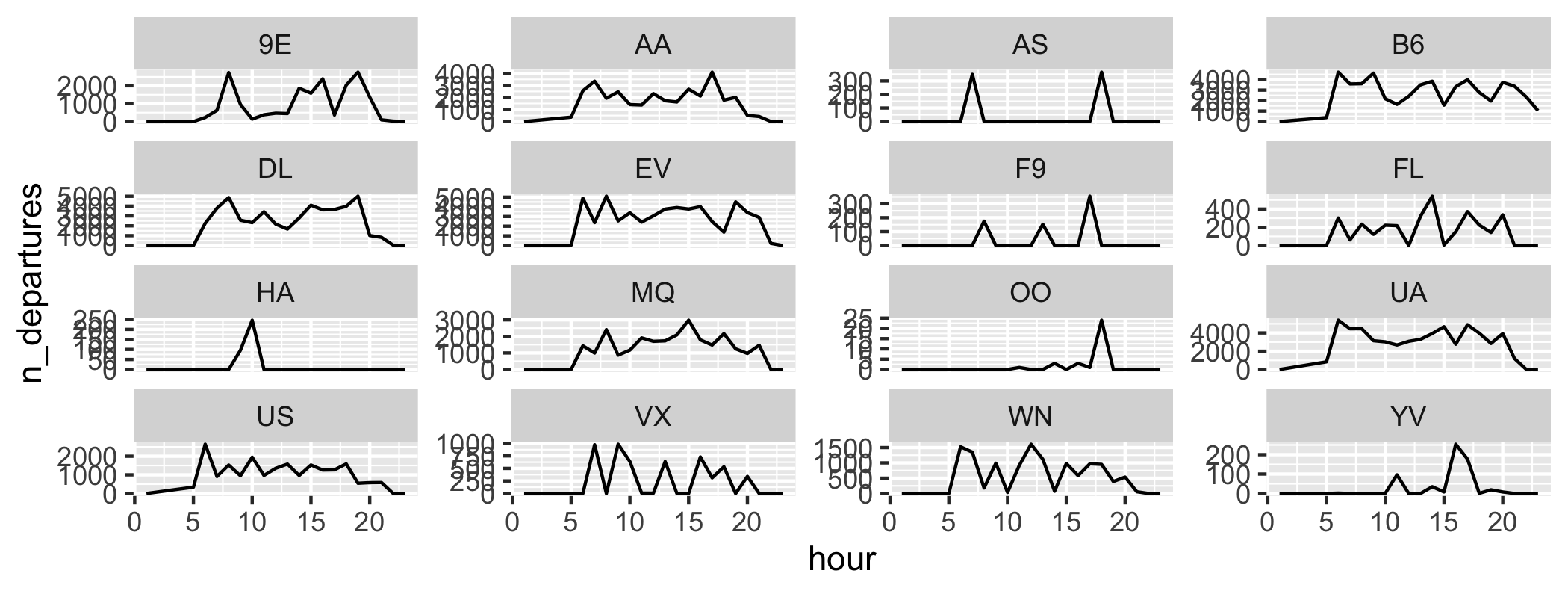<!-- --> --- By the way, `summarize` seems to group the output only by `carrier`? what about `hour`? ```r departures = flights %>% group_by(carrier, hour) %>% summarize(n_departures = n()) ``` ``` ## `summarise()` has grouped output by 'carrier'. You can override using the ## `.groups` argument. ``` When you call `summarize` it requires computing a summary over a group of values -- by default, `summarize` achieves this by dropping the last group (`hour` in this case). --- ## grouping is contagious > `summarise()` has grouped output by 'carrier'. You can override using the `.groups` argument. This is telling us that by default, the output will be grouped if we use it in another pipeline. To save screen real estate, I'm going to turn off this message going forward: ```r options(dplyr.summarise.inform = FALSE) ``` In general you should set `.groups` explicitly. --- ## `ungroup()` to remove grouping variables. .pull-left[ Default ```r ontime_drop = ontime %>% group_by(carrier, dest) %>% summarize(ontime_pct = mean(ontime, na.rm = TRUE)*100) ontime_drop %>% summarize(n_dest = n_distinct(dest)) ``` ``` ## # A tibble: 16 × 2 ## carrier n_dest ## <chr> <int> ## 1 9E 49 ## 2 AA 19 ## 3 AS 1 ## 4 B6 42 ## # ℹ 12 more rows ``` ] .pull-right[ ungrouped ```r *ontime_drop %>% ungroup() %>% summarize(n_dest = n_distinct(dest)) ``` ``` ## # A tibble: 1 × 1 ## n_dest ## <int> ## 1 105 ``` ] --- ## `group_by() filter()` We can combine group_by with filter, mutate or arrange to evaluate these verbs on each group. ```r ontime_1500 = ontime %>% group_by(dest) %>% filter(n() > 1500) %>% mutate(n_flights_dest = n(), .after = 1) ontime_1500 %>% arrange(n_flights_dest) ``` ``` ## # A tibble: 314,599 × 22 ## # Groups: dest [53] ## year n_flights_dest month day dep_time sched_dep_time ## <int> <int> <int> <int> <int> <int> ## 1 2013 1525 1 1 1304 1227 ## 2 2013 1525 1 1 1732 1630 ## 3 2013 1525 1 2 834 823 ## 4 2013 1525 1 2 1228 1229 ## # ℹ 314,595 more rows ## # ℹ 16 more variables: dep_delay <dbl>, arr_time <int>, ## # sched_arr_time <int>, arr_delay <dbl>, carrier <chr>, … ``` --- ## Carrier performance by destination ```r ontime_drop = ontime_1500 %>% group_by(dest, carrier) %>% summarize(ontime_pct = mean(ontime, na.rm = TRUE)*100) ggplot(ontime_drop, aes(y = ontime_pct, x = dest)) + geom_point() + coord_flip() + theme_minimal(base_size = 8) ``` 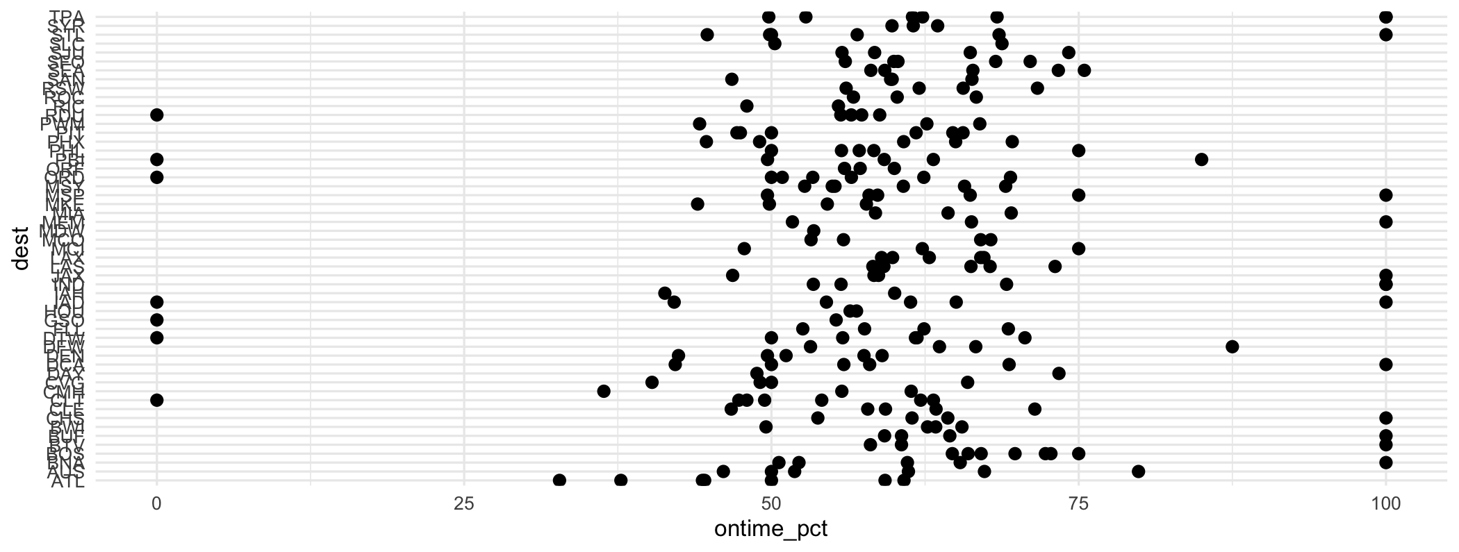<!-- --> --- ## The "law" of small numbers .question[What's with the carriers with 0% or 100% ontime percentages for a destination?] --- ## The "law" of small numbers ```r ontime_drop = ontime_1500 %>% group_by(dest, carrier) %>% summarize(ontime_pct = mean(ontime, na.rm = TRUE)*100, n_departed = sum(!is.na(ontime))) ggplot(ontime_drop, aes(y = ontime_pct, x = dest, color = n_departed<10)) + geom_point() + coord_flip() + theme_minimal(base_size = 8) ``` 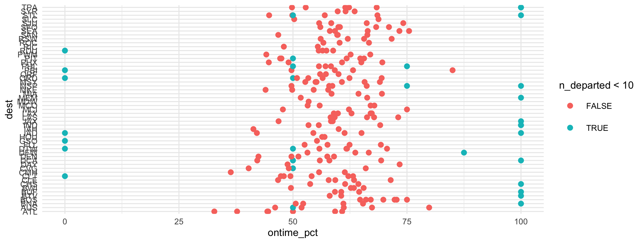<!-- --> .question[What are some statistical fixes to this issue?] --- ## Without small numbers ```r ontime_drop_10 = filter(ontime_drop, n_departed >= 10) ggplot(ontime_drop_10, aes(y = ontime_pct, x = dest)) + geom_boxplot() + coord_flip() + theme_minimal(base_size = 8) ``` 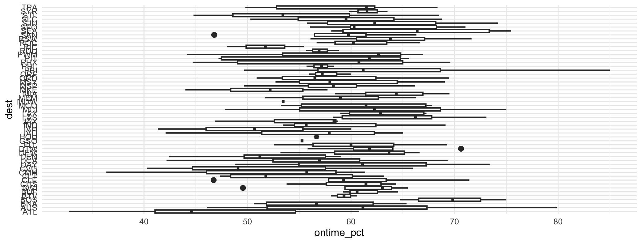<!-- --> Better...but it's hard to see the rank order of routes. --- ## A sensible plot order ```r ontime_drop_10 = ontime_drop_10 %>% ungroup() %>% * mutate(dest = forcats::fct_reorder(dest, ontime_pct)) ggplot(ontime_drop_10, aes(x = dest, y = ontime_pct)) + geom_boxplot() + coord_flip() + theme_minimal(base_size = 8) ``` <!-- --> We'll discuss the `fct_reorder` business in the coming weeks. --- ## `select()` <!-- 201 --> `select()` (as well as `pivot_wider()`, `pivot_longer()`, and friends) use [tidy-select](https://dplyr.tidyverse.org/reference/dplyr_tidy_select.html), which is a meta-language to select columns from a data frame. There are several helper functions you can use within `select()`: - `starts_with("abc")`: matches names that begin with "abc", - `ends_with("xyz")`: matches names that end with "xyz", - `contains("ijk")`: matches names that contain "ijk", - `num_range("x", 1:3)`: matches `x1`, `x2` and `x3`, - `last_col(offset = 0)`: last column, minus offset, - `where(<function>)`: columns where `<function>` returns `TRUE`, - `:` range, `c` concatenate, `!` negate, `&` intersect - ...and a few others. --- ## select delay columns ```r flights %>% select(ends_with('delay')) ``` ``` ## # A tibble: 336,776 × 2 ## dep_delay arr_delay ## <dbl> <dbl> ## 1 2 11 ## 2 4 20 ## 3 2 33 ## 4 -1 -18 ## # ℹ 336,772 more rows ``` --- ## everything except columns containing "time" ```r flights %>% select(!contains('time')) ``` ``` ## # A tibble: 336,776 × 14 ## year month day dep_delay arr_delay carrier flight ## <int> <int> <int> <dbl> <dbl> <chr> <int> ## 1 2013 1 1 2 11 UA 1545 ## 2 2013 1 1 4 20 UA 1714 ## 3 2013 1 1 2 33 AA 1141 ## 4 2013 1 1 -1 -18 B6 725 ## # ℹ 336,772 more rows ## # ℹ 7 more variables: tailnum <chr>, origin <chr>, ## # dest <chr>, distance <dbl>, hour <dbl>, minute <dbl>, … ``` --- ## character columns ```r flights %>% select(where(is.character)) ``` ``` ## # A tibble: 336,776 × 5 ## carrier tailnum origin dest delay_type ## <chr> <chr> <chr> <chr> <chr> ## 1 UA N14228 EWR IAH lost time ## 2 UA N24211 LGA IAH lost time ## 3 AA N619AA JFK MIA lost time ## 4 B6 N804JB JFK BQN life is good ## # ℹ 336,772 more rows ``` --- ## Columns with no missing values ```r flights %>% select(where(~!any(is.na(.x)))) ``` ``` ## # A tibble: 336,776 × 13 ## year month day sched_dep_time sched_arr_time carrier ## <int> <int> <int> <int> <int> <chr> ## 1 2013 1 1 515 819 UA ## 2 2013 1 1 529 830 UA ## 3 2013 1 1 540 850 AA ## 4 2013 1 1 545 1022 B6 ## # ℹ 336,772 more rows ## # ℹ 7 more variables: flight <int>, origin <chr>, ## # dest <chr>, distance <dbl>, hour <dbl>, minute <dbl>, … ``` The above uses a tidyverse way to define an **anonymous function** and is equivalent to ``` none_na = function(x) !any(is.na(x)) ``` --- class: middle .hand[# Repeating an operation with `across`] --- ## `across()` If you need to repeat the same operation on multiple columns, you can avoid many keystrokes by using across. The syntax is a bit idiomatic, but in general, it looks something like ```r verb(across(.cols = <tidy selection>, .funs = list(<fun1>, <fun2>, ...))) ``` where `verb` is `summarize`, `mutate`, and a few others where unquoted columns are provided to a transformation. --- ## NYC AirBNB data ```r nycbnb ``` ``` ## # A tibble: 12,773 × 16 ## id name host_id price neighborhood accommodates ## <dbl> <chr> <dbl> <dbl> <chr> <dbl> ## 1 2595 Skylit Midt… 2845 150 Midtown 1 ## 2 3831 Whole flr w… 4869 75 Bedford-Stu… 3 ## 3 5121 BlissArtsSp… 7356 60 Bedford-Stu… 2 ## 4 5136 Spacious Br… 7378 275 Sunset Park 4 ## # ℹ 12,769 more rows ## # ℹ 10 more variables: room_type <chr>, borough <chr>, ## # minimum_nights <dbl>, maximum_nights <dbl>, … ``` --- ## Nights ```r availability = nycbnb %>% group_by(neighborhood) %>% * summarize(across(c(maximum_nights, minimum_nights, availability_90), median)) ggplot(availability, aes(x = neighborhood, ymin = minimum_nights, y = availability_90, ymax = maximum_nights)) + geom_pointrange() + coord_flip() + theme_minimal() + labs(x = NULL, y = 'Availability (minimum, 90 day, maximum)') ``` --- ## Nights <!-- --> --- ## Transform by variable type This can be very powerful: ```r median_mad = nycbnb %>% group_by(neighborhood) %>% * summarise(across(where(is.numeric), * list(median = median, mad = mad))) glimpse(median_mad) ``` ``` ## Rows: 41 ## Columns: 23 ## $ neighborhood <chr> "Astoria", "Bedford-S… ## $ id_median <dbl> 26455688, 29970716, 3… ## $ id_mad <dbl> 22196285, 22187834, 1… ## $ host_id_median <dbl> 48372942, 39365482, 5… ## $ host_id_mad <dbl> 66969215, 56397777, 7… ## $ price_median <dbl> 75.0, 100.0, 75.0, 98… ## $ price_mad <dbl> 35.5824, 66.7170, 44.… ## $ accommodates_median <dbl> 2, 2, 2, 3, 2, 3, 2, … ## $ accommodates_mad <dbl> 1.4826, 1.4826, 1.482… ## $ minimum_nights_median <dbl> 14.0, 5.0, 5.0, 2.0, … ## $ minimum_nights_mad <dbl> 19.2738, 5.9304, 5.93… ## $ maximum_nights_median <dbl> 1125, 365, 365, 365, … ## $ maximum_nights_mad <dbl> 0.0000, 526.3230, 526… ## $ availability_90_median <dbl> 50.0, 38.0, 47.0, 70.… ## $ availability_90_mad <dbl> 41.5128, 40.0302, 40.… ## $ beds_median <dbl> NA, NA, NA, NA, NA, 1… ## $ beds_mad <dbl> NA, NA, NA, NA, NA, 1… ## $ review_scores_rating_median <dbl> 4.830, 4.800, 4.800, … ## $ review_scores_rating_mad <dbl> 0.252042, 0.266868, 0… ## $ number_of_reviews_median <dbl> 17.0, 20.0, 13.0, 17.… ## $ number_of_reviews_mad <dbl> 22.2390, 26.6868, 17.… ## $ number_of_reviews_ltm_median <dbl> 2.0, 2.0, 2.0, 4.0, 3… ## $ number_of_reviews_ltm_mad <dbl> 2.9652, 2.9652, 2.965… ``` --- # Resources - [Chapter 3 R4DS](https://r4ds.hadley.nz/data-transform.html) - [Chapter 12 R4DS](https://r4ds.hadley.nz/logicals.html) - [Chapter 13 R4DS](https://r4ds.hadley.nz/numbers.html) - [Data Transformation Cheat Sheet](https://github.com/rstudio/cheatsheets/blob/master/data-transformation.pdf). - [`dplyr` Overview](https://dplyr.tidyverse.org/). --- # Acknowledgments This lecture contains materials adapted from [Mine Çetinkaya-Rundel and colleagues](https://github.com/Sta199-S18/website/blob/master/static/slides/lec-slides/02b-tidy-data-wrangle.Rmd) and [David Gerard](https://github.com/URMC-BST/stat_412_612/blob/master/lectures/04_dplyr/04_dplyr.Rmd).