BST430 Lecture 15

Testing and High-throughput count data

Seong-Hwan Jun

2025-10-30

Hypothesis testing

Statistical hypothesis testing is a method used to make inferences or draw conclusions about a population based on sample data.
It involves formulating two competing hypotheses: the null hypothesis (\(H_0\)) and the alternative hypothesis (\(H_a\)).

Collect data

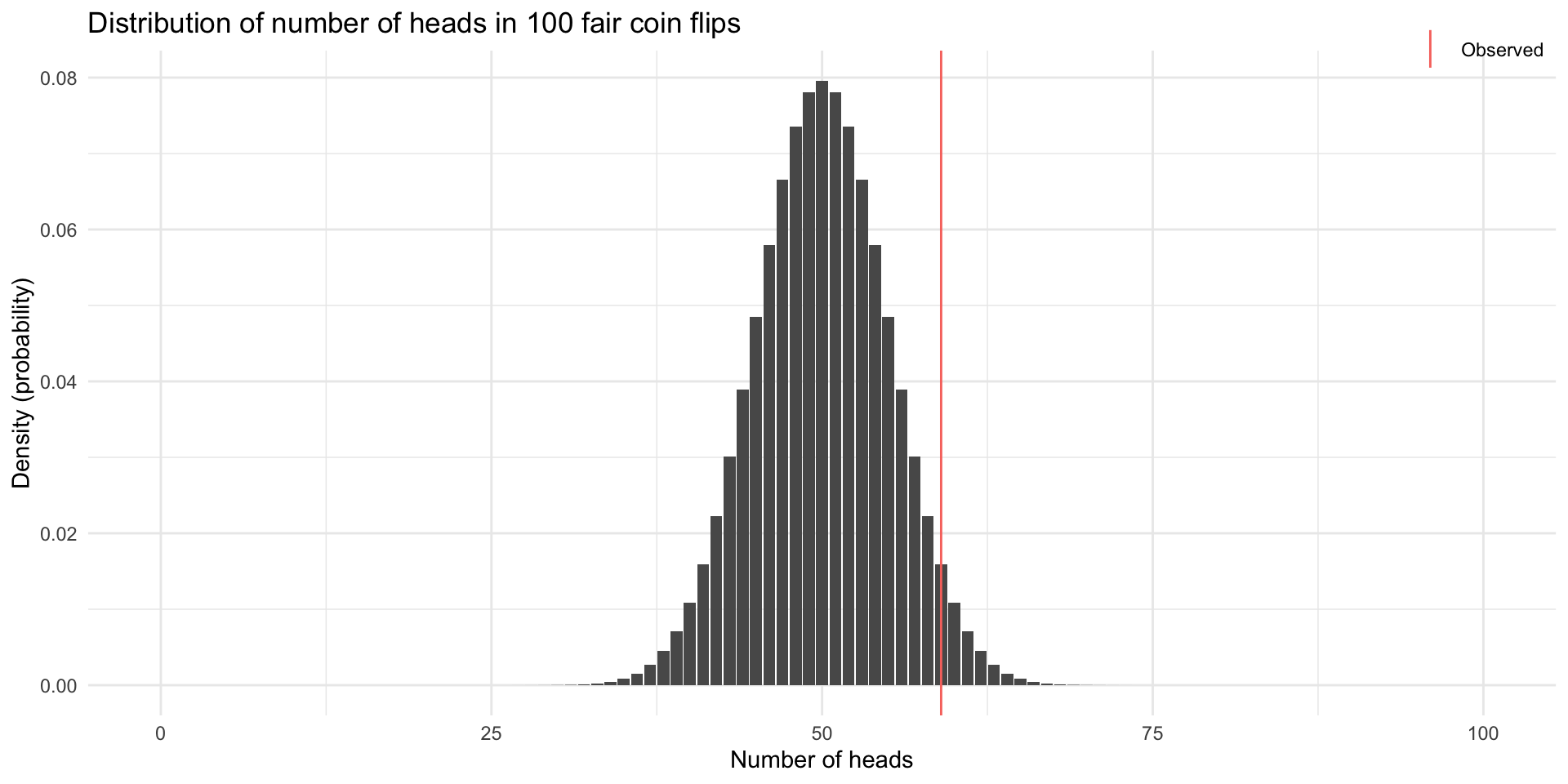
Example: coin flip.

\(X_i \sim \text{Bernoulli}(p)\), where \(p\) is the probability of getting heads.
Flip the coin \(n\) times and record the number of heads observed, denoted as \(X_i; i = 1, ..., n\).
How would you test if the coin is fair (\(H_0: p = 0.5\)) or biased (\(H_a: p \neq 0.5\))?

Test statistic

A test statistic is a numerical summary of the data that is used to evaluate the evidence against the null hypothesis.
It is calculated from the sample data and is used to determine the likelihood of observing the data under the null hypothesis.

If \(p = 0.5\) were true, how likely is it to observe the number of heads we did?

Generate some data

[1] "T" "T" "H" "T" "H" "H"

coinFlips
 H  T 
59 41

Binomial distribution under null

Rejection region

The rejection region is the range of values for the test statistic that leads to the rejection of the null hypothesis.
It is determined based on the significance level (\(\alpha\)) chosen for the test.
For a two-tailed test with \(\alpha = 0.05\), the rejection region would include values of the test statistic that are in the extreme 2.5% on either side of the distribution under the null hypothesis.

Rejection region

So we do not reject the null hypothesis. Does that mean the coin is fair?

Binomial test

binom.test(x = sum(coinFlips == "H"), n = numFlips, p = 0.5)


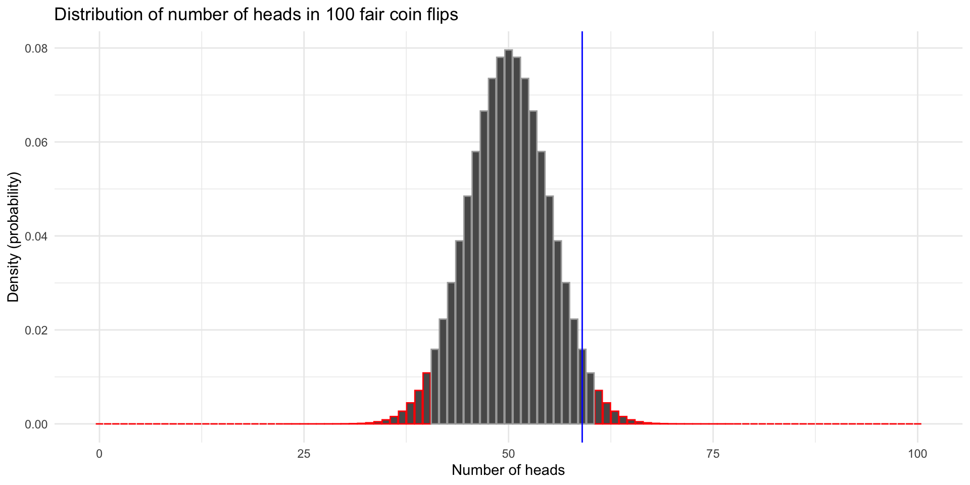
    Exact binomial test

data:  sum(coinFlips == "H") and numFlips
number of successes = 59, number of trials = 100, p-value = 0.08863
alternative hypothesis: true probability of success is not equal to 0.5
95 percent confidence interval:
 0.4871442 0.6873800
sample estimates:
probability of success 
                  0.59

Sample size

What if we increased the sample size to 1000 flips with the same probability of heads?

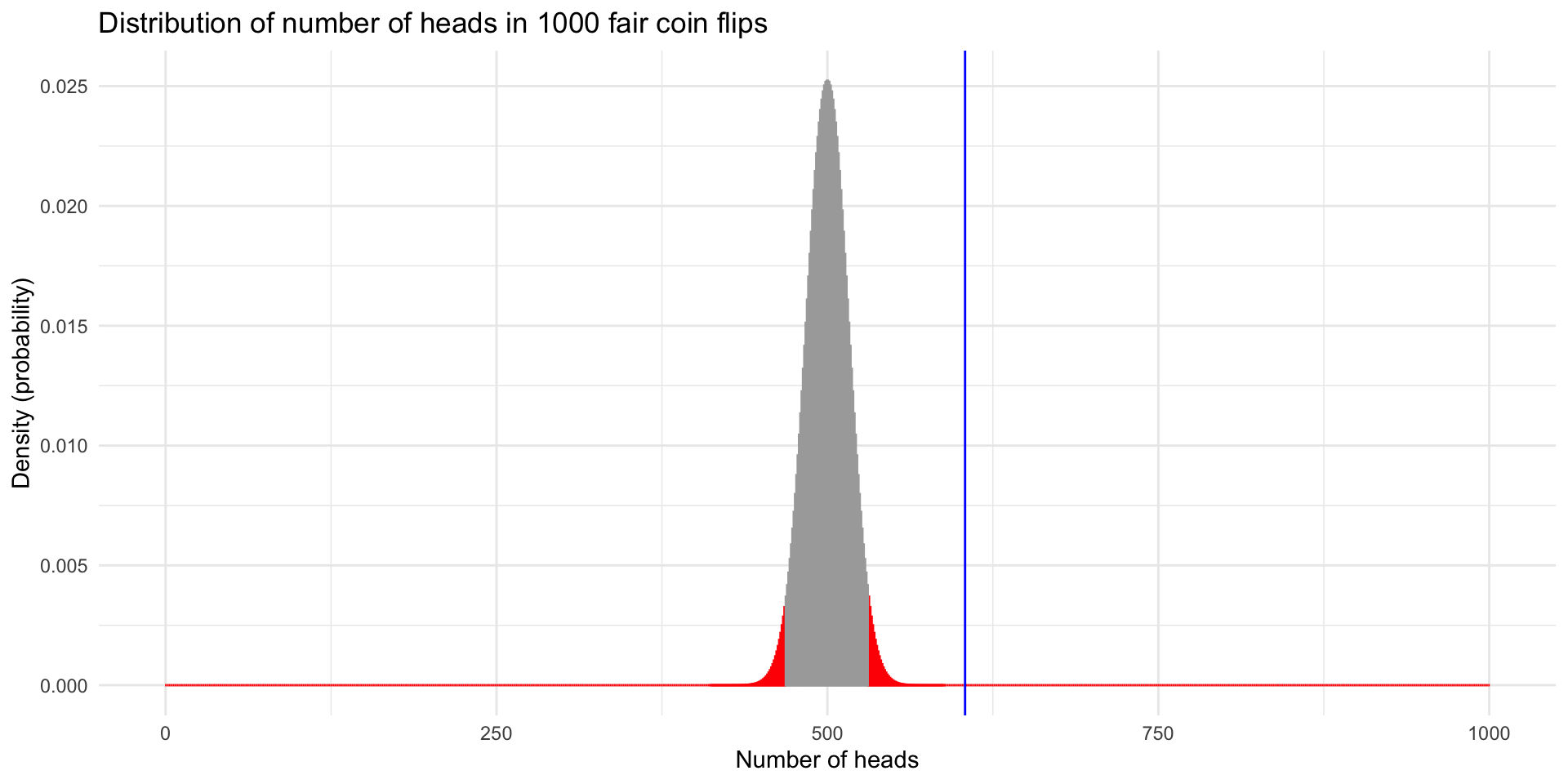
coinFlips
  H   T 
604 396

Binomial distribution under null

Binomial test

binom.test(x = sum(coinFlips == "H"), n = numFlips, p = 0.5)


    Exact binomial test

data:  sum(coinFlips == "H") and numFlips
number of successes = 604, number of trials = 1000, p-value = 5.062e-11
alternative hypothesis: true probability of success is not equal to 0.5
95 percent confidence interval:
 0.5729182 0.6344677
sample estimates:
probability of success 
                 0.604

Testing set up

Suppose we are interested in testing efficacy of a treatment (drug/procedure/etc).
A: Control/B: Treatment.
We collect a sample of size n from each group and measure some outcomes of interest (e.g., blood pressure, gene expression levels, etc).
We want to test whether there is a significant difference in the outcomes between the two groups.

High throughput sequencing data

High-throughput sequencing

High-throughput sequencing (HTS) technologies have revolutionized genomics and molecular biology.
Rapid sequencing of large volumes of DNA and RNA molecules.

Experimental set up

Biological samples are collected under different conditions (e.g., treatment vs. control or healthy vs disease).
The resulting data consists of counts of reads mapped to each genetic material of interest, e.g., gene, transcript, microbiome, etc.
We aim to identify genes that are differentially expressed between conditions to characterize disease progression or differences brought forth by treatment (efficacy).

Examples

Bulk RNA sequencing
- Measure gene expression levels in a population of cells.
- The resulting data consists of counts of transcripts for each gene aggregated over all cells captured.

Examples

Single-cell RNA sequencing
- Profile gene expression at the single-cell level.
- Cells are isolated, and their RNA is sequenced individually.
- The resulting data consists of counts of transcripts for each gene in each cell.
- Enables the study of cellular heterogeneity and identification of distinct cell types or states.

Examples

Genetic screening using RNAi or CRISPR-Cas9
- Identify genes essential for cell survival or proliferation.
- Cells are transduced with a library of RNAi or CRISPR constructs targeting different genes.
- After a period of growth, the abundance of each construct is measured using HTS.
- Counts reflect the impact of gene knockdown or knockout on cell viability.

Examples

Microbiome studies
- Abundance of microbiome (e.g., gut or oral microbiota) in maintaining health or contributing to disease.
- Samples are collected from different environments or conditions.

Statistical challenges

We observe a random sample of genetic molecules that are present in the sample (sequencing can be biased).
Data is count-based, often with many zeros (sparsity).
Noise and variability due to technical and biological factors. Examples, batch effects and other confounding factors.
High dimensionality with many genes and relatively few samples.
Multiple testing issues when identifying differentially expressed genes.
Complex dependencies among genes.

Bulk RNA-seq counts

library(pasilla)
fn = system.file("extdata", "pasilla_gene_counts.tsv",
                 package = "pasilla", mustWork = TRUE)
counts = as.matrix(read.csv(fn, sep = "\t", row.names = "gene_id"))
print(dim(counts))

[1] 14599     7

print(colnames(counts))

[1] "untreated1" "untreated2" "untreated3" "untreated4" "treated1"  
[6] "treated2"   "treated3"

head(rownames(counts))

[1] "FBgn0000003" "FBgn0000008" "FBgn0000014" "FBgn0000015" "FBgn0000017"
[6] "FBgn0000018"

Quiz

Compute the gene wise (rows) log of the means.
Plot the log of the mean. What plot type is appropriate to visualize the distribution of the means?

Quiz

genewise_vars <- rowVars(counts)
boxplot(log(genewise_vars))

# Focus on 2000 most variable genes.
num_genes <- 2000
genes_to_analyze <- names(sort(genewise_vars, decreasing = TRUE))[1:num_genes]
cts_subset <- counts[genes_to_analyze,]

Testing differential expression

We want to find genes that are differentially expressed between two conditions (treated vs untreated).
Testing over 10,000 genes (multiple testing) -> highly probable that we may find significant genes by chance (false discovery).
What test should we use?

Quiz

Try t.test on each gene between the two conditions.
Adjust for multiple testing using Benjamini-Hochberg procedure p.adjust(..., method="BH").
How many genes are significant at FDR 5%?
Are the assumptions of the t-test satisfied?

Permutation test

A permutation test is a non-parametric statistical test used to determine the significance of an observed effect.
It involves randomly shuffling the data to create a null distribution of the test statistic.
The p-value is calculated by comparing the observed test statistic to the null distribution.

When to use permutation tests

Why (or when) would we use this?

When the assumptions of traditional parametric tests (e.g., t-test, ANOVA) are not met.
When dealing with small sample sizes where parametric tests may not be reliable.

Quiz

How many random shuffling of the data points (permutations) are possible?
Write code to perform permutation test for one of the genes. Generate 10, 20, and all 35 permutations.
- What statistic should we compute?

Quiz

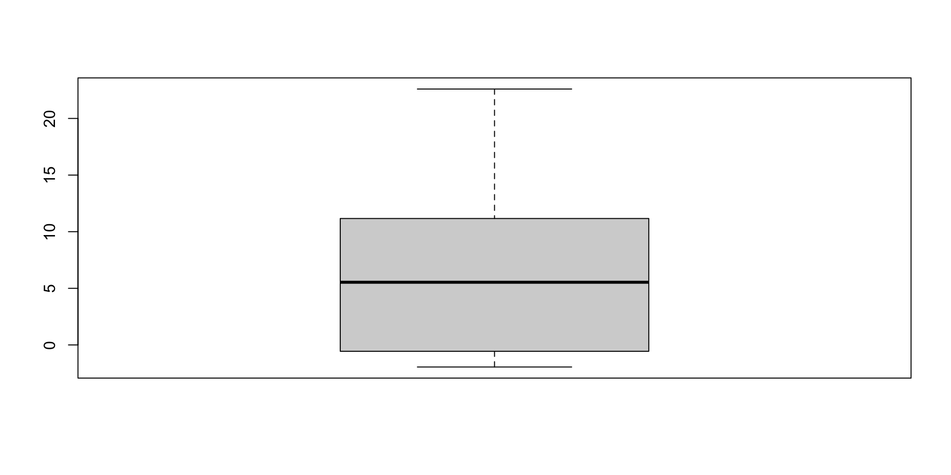
log_counts <- log1p(cts_subset)
gene <- genes_to_analyze[1]
shuffles <- combn(7, 4)
diffs <- apply(shuffles, 2, function(untreated_idx) {
  mean(log_counts[gene,untreated_idx]) - mean(log_counts[gene,-untreated_idx])
})
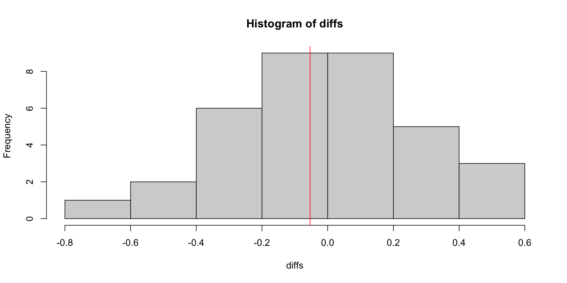
untreated_mean <- mean(log_counts[gene, str_detect(colnames(log_counts), "untreated")])
treated_mean <- mean(log_counts[gene, str_detect(colnames(log_counts), "treated")])
observed <- treated_mean - untreated_mean
print(observed)

[1] -0.05359491

p_value <- mean(abs(diffs) >= abs(observed))
print(p_value)

[1] 0.8571429

Quiz

hist(diffs)
abline(v=observed, col="red")

GLM for count-valued variables.

In the simple setting where you only have an experimental condition, non-parametric tests such as the permutation test or others (e.g., Wilcoxon rank sum test) may be fine.
If you have multiple conditions or covariates to adjust for (e.g., batch effects), you may want to consider a regression-based approach.
Since we have counts data, we can consider a Poisson or Negative Binomial Generalized Linear Model (GLM).

Fitting Poisson GLM

We will use glm(..., family = "poisson") to fit a Poisson GLM.
To facilitate ease of modeling we will group the data by gene and then use nest function.

Fitting Poisson GLM

Prepare the data…

dat <- data.frame(genes = rownames(cts_subset), cts_subset)
colnames(dat)

[1] "genes"      "untreated1" "untreated2" "untreated3" "untreated4"
[6] "treated1"   "treated2"   "treated3"

dat_long <- pivot_longer(dat, cols = -genes, names_to = "sample", values_to = "count") %>% 
  mutate(condition = if_else(str_detect(pattern = "untreated", sample), "untreated", "treated"))

# Nest data by genes
nested_data <- dat_long %>%
  group_by(genes) %>%
  nest()
nested_data

# A tibble: 2,000 × 2
# Groups:   genes [2,000]
   genes       data            
   <chr>       <list>          
 1 FBgn0000556 <tibble [7 × 3]>
 2 FBgn0064225 <tibble [7 × 3]>
 3 FBgn0040813 <tibble [7 × 3]>
 4 FBgn0002526 <tibble [7 × 3]>
 5 FBgn0000559 <tibble [7 × 3]>
 6 FBgn0026562 <tibble [7 × 3]>
 7 FBgn0000042 <tibble [7 × 3]>
 8 FBgn0027571 <tibble [7 × 3]>
 9 FBgn0001219 <tibble [7 × 3]>
10 FBgn0003517 <tibble [7 × 3]>
# ℹ 1,990 more rows

Fitting Poisson GLM

poisson_glm_nested <- nested_data %>% 
  mutate(glm = map(data, ~glm(count ~ condition, data = .x, family = "poisson")),
         tidy_glm = map(glm, broom::tidy))
poisson_glm_nested

# A tibble: 2,000 × 4
# Groups:   genes [2,000]
   genes       data             glm    tidy_glm        
   <chr>       <list>           <list> <list>          
 1 FBgn0000556 <tibble [7 × 3]> <glm>  <tibble [2 × 5]>
 2 FBgn0064225 <tibble [7 × 3]> <glm>  <tibble [2 × 5]>
 3 FBgn0040813 <tibble [7 × 3]> <glm>  <tibble [2 × 5]>
 4 FBgn0002526 <tibble [7 × 3]> <glm>  <tibble [2 × 5]>
 5 FBgn0000559 <tibble [7 × 3]> <glm>  <tibble [2 × 5]>
 6 FBgn0026562 <tibble [7 × 3]> <glm>  <tibble [2 × 5]>
 7 FBgn0000042 <tibble [7 × 3]> <glm>  <tibble [2 × 5]>
 8 FBgn0027571 <tibble [7 × 3]> <glm>  <tibble [2 × 5]>
 9 FBgn0001219 <tibble [7 × 3]> <glm>  <tibble [2 × 5]>
10 FBgn0003517 <tibble [7 × 3]> <glm>  <tibble [2 × 5]>
# ℹ 1,990 more rows

Fitting Poisson GLM

p_values <- poisson_glm_nested %>%
  unnest(tidy_glm) %>% 
  filter(term == "conditionuntreated") %>%
  dplyr::pull(p.value)
# Adjust for multiple testing.
adj_pvalues <- p.adjust(p_values, method = "BH")
# Number of differential genes.
sum(adj_pvalues < 0.05)

[1] 1704

A bit too many?

Diagnostics

Poisson distribution assumes that the mean and variance are equal.

Diagnostics

Negative Binomial GLM

To account for overdispersion, we can use a Negative Binomial GLM.
Negative Binomial distribution has two parameters, one parameter to account for dispersion.
We will need to use glm.nb from MASS package (not offered by glm).

Negative Binomial GLM

nb_glm_nested <- nested_data %>% 
  filter(genes %in% genes_to_analyze) %>% 
  mutate(glm = map(data, ~glm.nb(count ~ condition, data = .x)),
         tidy_glm = map(glm, broom::tidy))
p_values <- nb_glm_nested %>%
  unnest(tidy_glm) %>% 
  filter(term == "conditionuntreated") %>%
  dplyr::pull(p.value)
adj_pvalues <- p.adjust(p_values, method = "BH")
sum(adj_pvalues < 0.05)

[1] 11

Quiz

Compare the counts (or log counts) of untreated vs treated for the genes that are selected as differentially expressed by Negative Binomial GLM.
Do you think these are truly differential?

Note

We actually did not account for library size differences between samples here.
In practice, we would want to include an offset term in the GLM to account for library size differences.
More sophisticated methods such as edgeR and DESeq2 elicit prior on dispersion parameter by pooling information across genes.