Probabilistic Machine Learning

Overview

Seong-Hwan Jun

Department of Biostatistics and Computational Biology, University of Rochester Medical Center

Logistics

BST 570-1 Probabilistic Machine Learning (4 credits)

• Lectures: Monday/Wednesday 1:30PM - 2:40PM.
• Tutorial/Lab: Thursday 1:30PM - 2:20PM.
• Location: SRB 1.404.
• Office hour: By appointment.

Note

Assumed background: probability at the level of a first graduate course, linear algebra (matrices, eigendecomposition). No Python experience is assumed – that is what the labs are for.

Course objectives

• Learn to formulate custom probabilistic models for real world problems.
• Understand the principles of probabilistic reasoning.
• Gain familiarity with inference and learning methods.
• Gain familiarity with machine learning software libraries and add Python to your research toolbox.

Textbooks

Primary, both by Kevin Murphy and free to download:

• Probabilistic Machine Learning: An Introduction (PML1).
• Probabilistic Machine Learning: Advanced Topics (PML2).

Also useful:

• Machine Learning: a Probabilistic Perspective (MLPP), Murphy. Older, but combines most of PML1 and PML2 into one volume.
• Pattern Recognition and Machine Learning (PRML), Bishop. Free PDF; the classic treatment of graphical models and message passing.

Outline

• Foundation
• Exact Inference
• Exactly Approximate Inference
• Approximately Approximate Inference
• Topics and trends in probabilistic machine learning

Roughly week by week

week	topic
1	Overview
2	Probability and Bayesian inference
3	Mixture models and the EM algorithm
4	Hidden Markov models; forward-backward
5	Tree structured models; belief propagation; phylogenetics
6	Factor graphs; sum-product and max-product
7+	Sampling: MCMC and sequential Monte Carlo
11+	Variational inference, the ELBO, VAEs

The first half is exact inference: problems where we can compute the answer. The second half is what to do when we cannot.

Assessment

• 40% assignments (5-6 over the term).
  • One problem broken into subproblems.
  • Each student presents part of their solution in class.
• 10% x 2 quizzes, multiple choice questions.
  • Quiz 1 once we finish exact inference (around week 6 or 7).
  • Quiz 2 at the end of the semester.
• 10% labs, graded for completion and participation.
• 30% paper presentation.
  • Read a research paper closely and present it to the class.
  • Critically read and assess machine learning research.
  • Presentations take place during the semester, in the week the paper’s topic is covered in lecture.

Paper presentation: reading list (1/3)

Pick one paper. You present it in the week its topic is covered, so papers on early topics need to be claimed early.

Message passing (week 6).

• Belief propagation and its generalizations. Yedidia, J. S., Freeman, W. T., and Weiss, Y. (2003). Understanding belief propagation and its generalizations. In Lakemeyer and Nebel (eds.), Exploring Artificial Intelligence in the New Millennium, Ch. 8, 239–269. Morgan Kaufmann.

Markov chain Monte Carlo Sampling (week 8).

• Hamiltonian Monte Carlo. Neal, R. M. (2011). MCMC using Hamiltonian dynamics. In Brooks, Gelman, Jones, and Meng (eds.), Handbook of Markov Chain Monte Carlo, Ch. 5. arXiv:1206.1901.
• Dirichlet process mixtures. Neal, R. M. (2000). Markov chain sampling methods for Dirichlet process mixture models. JCGS, 9(2), 249–265.

Paper presentation: reading list (2/3)

Sequential Monte Carlo Sampling (week 11).

• Particle filters for HMMs. Fearnhead, P. and Clifford, P. (2003). On-line inference for hidden Markov models via particle filters. JRSS-B, 65(4), 887–899.
• SMC samplers. Del Moral, P., Doucet, A., and Jasra, A. (2006). Sequential Monte Carlo samplers. JRSS-B, 68(3), 411–436.
• Particle MCMC. Andrieu, C., Doucet, A., and Holenstein, R. (2010). Particle Markov chain Monte Carlo methods. JRSS-B, 72(3), 269–342.
• SMC for phylogenetics. Bouchard-Côté, A., Sankararaman, S., and Jordan, M. I. (2012). Phylogenetic inference via sequential Monte Carlo. Systematic Biology, 61(4), 579–593.

Paper presentation: reading list (3/3)

Variational inference (week 14).

• LDA. Blei, D. M., Ng, A. Y., and Jordan, M. I. (2003). Latent Dirichlet allocation. JMLR, 3, 993–1022.
• Variational autoencoders. Kingma, D. P. and Welling, M. (2014). Auto-encoding variational Bayes. ICLR. arXiv:1312.6114.
• Normalizing flows. Rezende, D. J. and Mohamed, S. (2015). Variational inference with normalizing flows. ICML, PMLR 37, 1530–1538.

What is machine learning?

According to Tom Mitchell (CMU professor):

A computer program is said to learn from experience \(E\) with respect to some class of tasks \(T\) and performance measure \(P\), if its performance at tasks in \(T\), as measured in \(P\), improves with experience \(E\).

• \(E\), experience, is essentially data. What are the common data types and structures?
• Examples of \(P,T\)?

Supervised learning

• \(E = \{(x_i, y_i)\}_{i=1}^{N}\) where \(x_i \in \mathcal{X}\) and \(y_i \in \mathcal{Y}\).
• \(\mathcal{X}\) denotes the input space, usually represented in a tabular form (\(N \times D\) matrix – e.g., design matrix).
• \(\mathcal{Y}\) denotes the output space.
• The goal is to “learn” a mapping:

\[\begin{align} f : \mathcal{X} \to \mathcal{Y}. \end{align}\]

Here, “learn” means to find \(f\) that optimizes performance measure \(P\) at task \(T\). How?

Example: regression

Let \(\mathcal{Y} = \mathbb{R}\) and define a quadratic loss for each \((x_i, y_i) \in E\):

\[\begin{align} \mathcal L(E) = \sum_i (f(x_i) - y_i)^2 \end{align}\]

A computer program is said to learn from experience \(E\) with respect to some class of tasks \(T\) and performance measure \(P\), if its performance at tasks in \(T\), as measured in \(P\), improves with experience \(E\).

Performance \(P\) at task \(T\) needs to improve with experience \(E\)… how do we ensure this?

Let us further assume \(f\) is a linear function of \(x \in \mathcal{X}\):

\[\begin{align} f_{\beta}(x) = \beta^T x, \end{align}\]

then by minimizing \(\mathcal L(E)\), we are optimizing the parameters \(\beta\) of the linear model.

Essentially, learning in this context amounts to solving a linear regression problem:

\[ \hat{\beta} = \operatorname{argmin}_{\beta} \sum_i (f_{\beta}(x_i) - y_i)^2 \]

But how do we ensure that the performance \(P\) at task \(T\) improves with (additional) experience \(E\)?

Important

What does it mean for the performance \(P\) to improve on the task \(T\)? And, we didn’t specify what \(T\) is exactly.

Define \(T\) as prediction on unseen data:

\[ T : x_{\operatorname{new}} \mapsto \hat{y}_{\operatorname{new}} \]

Split \(E\) into train and test set. Let \(\mathcal D_{\operatorname{train}}, \mathcal D_{\operatorname{test}} \subset E\) denote the training and test data such that,

\[ \mathcal D_{\operatorname{train}} \cap \mathcal D_{\operatorname{test}} = \emptyset, \]

Optimize \(\mathcal L(f)\) on \(\mathcal{D}_{\operatorname{train}}\) to find \(f\) (for linear model, this amounts to finding \(\hat{\beta}\)).

Now, define \(P(f)\):

\[ P(f) = \sum_{(x_i, y_i) \in \mathcal D_{\operatorname{test}}} (f(x_i) - y_i)^2. \]

We do not directly optimize \(P(f)\) so how do we know that this procedure or learning algorithm improves on the future data?

Learning as generalization

Let’s assume that the dataset come from some distribution \(p\):

\[ (x, y) \sim p_{X,Y}. \]

If we can further assume that any new data \((x_{\operatorname{new}}, y_{\operatorname{new}}) \sim p_{X,Y}\), then

it is reasonable to expect that minimizing the training error produce good predictions on new observations.

Example: classification

• Let \(\mathcal{Y}\) be a discrete set.
• If \(\mathcal{Y} = \{0, 1\}\), we have a binary classification problem.
• If \(\mathcal{Y} = \{1, ..., K\}\), we have a multi-class classification problem.
• \(E = \{(x_i, y_i)\}\) as before.
• What are some of the choices for \(f\), \(\mathcal L\), \(P\), and \(T\)?

Example: binary classification

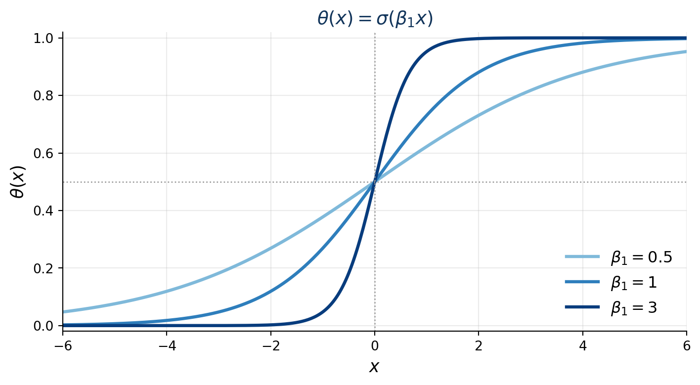
Let \(\mathcal{Y} = \{0, 1\}\) and we assume that \(y_i | x \sim \text{Bernoulli}(\theta(x))\), then we may choose the sigmoid function:

\[\begin{align} \theta(x) = f_{\beta}(x) = \frac{\exp(\beta^T x)}{1 + \exp(\beta^T x)}, \end{align}\]

and

\[\begin{align} \mathcal L(E) = \prod_i \theta_i^{y_i} (1 - \theta_i)^{1 - y_i}. \end{align}\]

In this case, \(\mathcal L\) is a likelihood and we are essentially fitting a logistic regression model:

\[ \hat{\beta} = \operatorname{argmax}_{\beta} \prod_{i=1}^{N} p(y_i | x_i, \beta). \]

The sigmoid \(\sigma(s) = e^s/(1+e^s)\) squashes the linear score \(s = \beta^\top x\) into \((0, 1)\); \(\theta(x) = 0.5\) is the decision boundary.

What about \(P\) and \(T\)?

Several choices (select one or all):

• Classification accuracy;
• Test log likelihood;
• Area under the ROC curve;
• Sensitivity and specificity;
• Others?

Note

The performance will vary depending on the choice of the loss function \(\mathcal L\) and the class of functions \(f \in \mathcal F\).

Learning as generalization: risk

Population risk:

\[ R(f) = \mathbb E_{(X, Y) \sim p}[\mathcal L(f(X), Y)]. \]

• Implicitly, using the training set, we were optimizing an empirical risk, e.g.,

\[ R_{\operatorname{train}}(f) = -\frac{1}{N} \sum_{i=1}^{N} \log p(y_i | x_i, \beta), \] and \(f\) is selected to optimize the risk (minimize).

• As \(N\) grows, we can reasonably expect \(R_{\operatorname{train}}(f)\) to approach \(R(f)\).
• Test set does not ensure generalization – but it does provide an (unbiased) estimate of the generalization performance.
• Generally, we also include validation set to guide in selecting any model hyperparameters so \(E = \{\mathcal D_{\operatorname{train}}, \mathcal D_{\operatorname{validation}}, \mathcal D_{\operatorname{test}} \}\).

Remarks

• Traditionally, ML has focused on the problem of optimizing \(f\).
  • Linear models, generalized linear models, support vector machines, random forests, deep neural networks, and etc are examples of such \(f\).
  • Performance on unseen data varies depending on the class of functions \(\mathcal{F}\).
  • Very complex \(\mathcal{F}\) is generally harder to train and requires more data to generalize.
• Most recent and advanced class is arguably the transformer architecture.
  • The large language models are trained on trillions of tokens.
  • We generally don’t have the scale of the data needed to use transformer for all of our problems.
• There’s still a lot of research to be done regarding selection and development of the models in machine learning specific to individual problems and data.

Unsupervised learning

• In many cases the label may be hard to obtain or unavailable – so \(E = \{ x_i \}_{i=1}^{N}\).
• We can think of the label as being hidden (latent) and infer its value: clustering.
• If \(x\) is high-dimensional, we may wish to learn the low dimensional embedding \(z\) that underlies \(x\): dimension reduction.

Note

In both cases there is a quantity \(z\) we never observe but want to reason about. That is the latent variable, and most models in this course have one.

What is probabilistic machine learning?

Generative models

• In a nutshell, what we are after is to “learn” the underlying data generating process.
• A generative model is a joint probability distribution with some observed and some latent/hidden.
• To specify the generative model, it is sufficient to specify the conditional distributions.
• The goal of this course is to build probabilistic models of data and develop algorithms for inference, prediction, and generation.

Generally speaking, we can separate the quantities into three components.

• Observed data: \((x, y)\)
• Latent variables: \(z\)
• Parameters: \(\theta\).
• We want to find a joint model \(p(x, y, z, \theta)\) to approximate the data generating process (assuming that the true data generating process is complex enough that we cannot deterministically model).

The same picture, every time

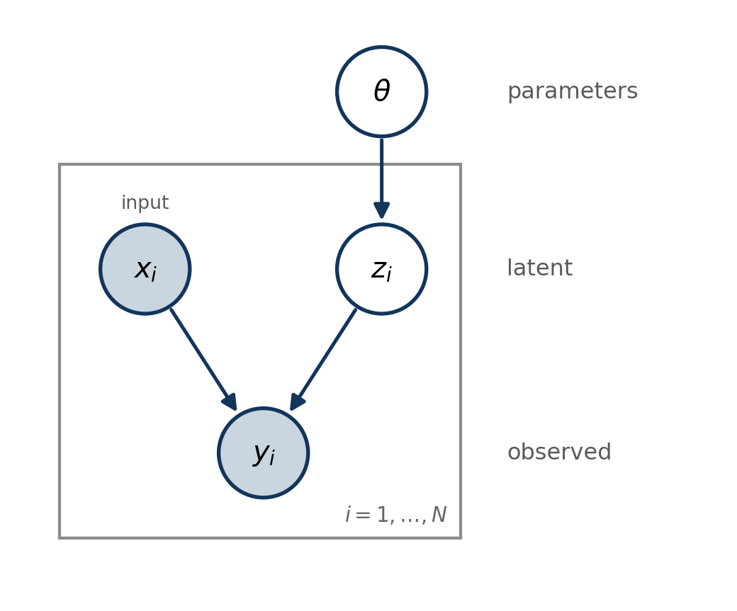
\[ p(x, y, z, \theta) = p(\theta) \prod_{i=1}^{N} p(x_i) \, p(z_i \mid \theta) \, p(y_i \mid x_i, z_i) \]

How to read it

• Shaded nodes are observed; unshaded are unknown. The inputs \(x_i\) and outputs \(y_i\) are shaded, and everything we want (\(z_i\) and \(\theta\)) is not.
• Arrows point from cause to effect – the direction the data were generated.
• The box is a plate: repeat its contents \(N\) times. \(\theta\) sits outside, because it is shared by every observation.

The model is written forwards, from \(\theta\) down to \(y\). Every question we care about runs backwards: we see \((x, y)\) and want \(z\) and \(\theta\). That reversal is what Bayes’ theorem does, and doing it efficiently on larger versions of this picture is the entire course.

Note

You will see this diagram again with the plate holding a mixture component, a Markov chain, or an evolutionary tree. The notation stays the same throughout.

Once we have a model…

There are three questions we can ask.

1. Inference;
2. Prediction;
3. Generation.

Inference

What hidden quantities explain my observations?

\[ p(z, \theta | x, y). \]

Examples:

• Which cluster does this observation belong to?
• What are the regression coefficients?

Note

Note that we are not after a single quantity \(z\) or \(\theta\) but a probability distribution around these quantities. In other words, we want uncertainty quantification via probabilistic modeling.

Inference and learning

What does it mean to “infer” and “learn”?

• Infer in this course generally means to compute the posterior distribution over the hidden variables \(z\).
• Learn is used for the (hyper)parameters \(\theta\): how to learn or estimate the parameters, e.g., point estimates.

Given observations \(x\), hidden variables \(z\), and parameters \(\theta\): how do we estimate \(\theta\) while accounting for the uncertainty in \(z\)?

Prediction

Given the experience \(E\) (our data),

What will happen next?

\[ p(y_{\operatorname{new}} | x_{\operatorname{new}}, E) \]

• Notice that this is itself a probability distribution.
• This is a key philosophical point.
• Classical ML predicts \(\hat{y}_{\operatorname{new}}\) as a point estimate,
• PML is interested in the distribution of \(y_{\operatorname{new}}\).

Generation

We can now generate new data from the model:

\[ x, y \sim p(x, y | \theta). \]

Examples from this course:

• Simulating new observations from a fitted mixture model (week 3);
• Sampling sequences from a hidden Markov model (week 4);
• Variational autoencoders (week 11+).

Probabilistic machine learning

• Relies on probability theory to specify relationship between random variables and model uncertainty.
• Probabilistic graphical models serve as a modeling language.
• Probabilistic reasoning via Bayesian statistics and computational techniques.
• Development of software libraries in the last decade has allowed for wide array of custom model specification and ease of inference (almost automatic!).

Note

Every algorithm we study – belief propagation, MCMC, variational inference, Hamiltonian Monte Carlo, and VAEs – is simply a different way of performing inference in probabilistic models.

Why Bayesian?

What is probability?

“Probability does not exist.” — Bruno de Finetti

• Probability is not an intrinsic property like mass or temperature.
• Probability represents uncertainty, or degree of belief given available information.

Two people with different information assign different probabilities to the same event, and neither is wrong. A card face down on the table is a definite card; your uncertainty about it is not a property of the card.

Example: Monty Hall problem

Famous game show:

• A car is hidden behind one of \(N = 3\) doors; a goat behind each of the other two.
• You pick a door. Call it \(i\).
• The host, who knows where the car is, then opens \(N - 2\) doors, never opening your door \(i\) and never opening the door hiding the car.
• Exactly one door other than yours is left closed. Call it \(j\).

Should you switch from \(i\) to \(j\)?

Important

Everything turns on the host’s rule. The host is not opening doors at random: the choice is constrained by knowledge you do not have, and that constraint is what makes the observation informative.

If the car is behind \(i\), the host chooses door \(j\) at random.

What is the probability that the car is behind each door?

• Without any further information, as a contestant, we formulate our belief that the car is behind the \(n\)-th door with probability \(1/3\).
• But in reality, the car is behind exactly one door, i.e., it’s not physically split across the three doors.
• As the show host, your belief that the car is behind the \(n\)-th door is \(1\) or \(0\).

Monty Hall with 10,000 doors

Let \(N = 10{,}000\).

Prior belief: you do not have any information so the car is equally likely to be behind each door: \(1/N\).

You choose door no. 1.

Observation: host opens all of the doors except door no. 1 and no. 387.

Is your belief on where the car is hidden updated? How would you update your belief?

Mechanism for updating beliefs

• Being Bayesian usually means that the performance measure is going to be the posterior distribution.
• Computing the posterior captures the inherent uncertainty associated with the variable.

Let \(H_n\) represent the hypothesis that the car is behind door \(n\).

Let \(Y \in \{1, ..., N\}\) denote the observation: which door is not opened by the show host.

Derive the posterior:

\[ P(H_n | Y = j). \]

\[ P(H_n | Y = j) = \frac{P(Y = j | H_n) P(H_n)}{P(Y = j)}. \]

• The prior:

\[ P(H_n) = 1/N. \]

What is \(P(Y = j | H_n)\)?

Note

We stop here on purpose. Work out the likelihood and the posterior before next week; we finish the derivation in lecture 2.

Why does this matter?

Two ways to read a probability

• Frequentist: a probability is a long run frequency. It attaches to repeatable events, not to fixed unknowns. “The car is behind door 387” is either true or false, so it has no probability.
• Bayesian: a probability is a degree of belief given the information you hold. Fixed unknowns get distributions, because your uncertainty about them is the thing being described.

Probability lives in the relationship between a question and the information available, not in the object itself. Monty Hall is exactly this: the game show host and the contestant assign wildly different probabilities to the same door, and both are correct.

Why this course takes the Bayesian view

• Our models have latent variables – cluster memberships, hidden states, ancestral sequences. These are fixed unknowns, exactly the objects a frequentist framework declines to put a distribution on.
• Almost everything we do reduces to computing a posterior \(p(z \mid x)\). Clustering, decoding a sequence, reconstructing an ancestor: same question, different graph.
• Uncertainty is often the answer, not a caveat. “Which cluster?” deserves a distribution, not a label – particularly in clinical settings.
• Prior information is real. Small samples plus domain knowledge is the normal situation in biostatistics.

The cost is computational: posteriors are usually intractable. That difficulty is the subject of this course.

Summary

• We are interested in the generative model: \(p(\text{hidden}, \text{observed})\) or \(p(\text{data}, \text{label})\).
  • This is in contrast to discriminative models that aim to learn \(p(\text{label} \mid \text{data})\).
• Graphical models serve as a modeling language, but also help you clarify the dependence structure and design inference algorithms.
• Bayesian statistics makes it natural to update your belief given observations.
• We will follow the development of probabilistic machine learning from mixture models and graphical models up to modern deep generative models such as variational autoencoders.

Notation

• Although we used \(P\) to refer to the performance metric, we will use \(L\) for loss moving forward.
• \(p\) is reserved for probability distributions (densities and mass functions).
• \(P\) is reserved for probability measures, e.g., \(P(H_n \mid Y = j)\).

Readings

• Introduction (PML1 Ch1 and PML2 Ch 1).
• Probability (PML2 Ch 2.1).
• Statistics (PML2 Ch 3.1-3.2)

For next class

• Install Visual Studio code (VS code)
• Install VS code extensions:
  • Python
  • Jupyter
  • Quarto
• Install miniforge.
  • If you already have a conda installed on your computer, you can keep miniforge installation.