Probabilistic Machine Learning

Lab 2: numpy, scipy, and Monte Carlo integration

Seong-Hwan Jun

Department of Biostatistics and Computational Biology, University of Rochester Medical Center

Where this fits

In lecture you computed the marginal likelihood of the coin flip in closed form:

\[ p(y_{1:N}) = \int_0^1 \theta^{s} (1-\theta)^{N-s} \, p(\theta) \, d\theta = \frac{B(s + a,\; N - s + b)}{B(a, b)}. \]

• That worked because Beta and Bernoulli are conjugate. Almost nothing else in this course will be so obliging.
• Today: compute the same integral by sampling, check it against the closed form, and then find out where the naive approach falls apart.

Goals

• numpy to generate random samples, scipy.stats to evaluate densities.
• Monte Carlo integration: turning an integral into an average.
• Why you must work on the log scale, demonstrated rather than asserted.
• Importance sampling: what to do when the thing you care about almost never happens.

Sampling and densities

Two libraries, two jobs

import numpy as np
import scipy.stats as ss

rng = np.random.default_rng(2)

x = rng.normal(loc=1.0, scale=2.0, size=5)      # numpy generates
print("samples:", np.round(x, 3))

print("pdf :", np.round(ss.norm.pdf(x, loc=1.0, scale=2.0), 4))   # scipy evaluates
print("cdf :", np.round(ss.norm.cdf(x, loc=1.0, scale=2.0), 4))
print("logpdf:", np.round(ss.norm.logpdf(x, loc=1.0, scale=2.0), 4))

samples: [ 1.378 -0.045  0.174 -3.883  4.599]
pdf : [0.1959 0.174  0.1832 0.0101 0.0395]
cdf : [0.575  0.3006 0.3398 0.0073 0.964 ]
logpdf: [-1.63   -1.7487 -1.6974 -4.5925 -3.2316]

Note

scipy.stats can sample too (ss.norm.rvs), and numpy can do most standard distributions. Use rng for sampling so your seed controls everything, and scipy for densities – especially logpdf, which you will need constantly.

Three idioms you will use today

x = rng.normal(size=6)
print("x        :", np.round(x, 2))

# 1. arithmetic with a scalar applies to every entry
print("x**2 * 3 :", np.round(x**2 * 3, 2))

# 2. a comparison gives a boolean array; True counts as 1, so .mean() is a fraction
print("x > 0    :", x > 0)
print("fraction :", (x > 0).mean())

# 3. build up results in a list, then hand it to numpy
results = []
for seed in range(3):
    r = np.random.default_rng(seed)
    results.append(r.normal(size=1000).mean())
print("results  :", np.round(np.array(results), 4))

x        : [ 1.14 -0.33  0.77  0.28 -0.55  0.98]
x**2 * 3 : [3.93 0.32 1.8  0.24 0.92 2.87]
x > 0    : [ True False  True  True False  True]
fraction : 0.6666666666666666
results  : [-0.048  -0.0543 -0.0224]

Task 1: get comfortable

rng = np.random.default_rng(0)

# TODO: draw 10,000 samples from Beta(2, 5)
# TODO: check the sample mean against the theoretical mean a/(a+b)
assert abs(samples.mean() - 2/7) < 0.01

# TODO: evaluate the Beta(2,5) density on a grid over [0,1] and plot it,
#       with a histogram of your samples (use density=True) behind it

Monte Carlo integration

Integrals are expectations

If \(p\) is a probability density that you can sample from, then

\[ I = \int f(\theta) \, p(\theta) \, d\theta = \mathbb{E}_{p}[f(\theta)] \]

can be estimated by drawing \(\theta_1, \ldots, \theta_K \sim p\) and averaging:

\[ \hat{I}_K = \frac{1}{K}\sum_{k=1}^{K} f(\theta_k). \]

• Law of large numbers: \(\hat I_K \to I\) as \(K \to \infty\) whenever \(\mathbb{E}_p|f(\theta)| < \infty\). That is why Monte Carlo works at all. It is also unbiased for every \(K\).
• Central limit theorem: if \(\operatorname{Var}_p(f) < \infty\), then \(\operatorname{sd}(\hat I_K) = \operatorname{sd}_p(f)/\sqrt{K}\) and the error is approximately normal. The rate is \(1/\sqrt{K}\) regardless of dimension, and that is why we do this at all.
• The catch is the constant. \(\operatorname{sd}_p(f)\) can be enormous, or infinite, in which case the rate claim is simply false.

The coin flip, again

\[ p(y_{1:N}) = \int_0^1 \underbrace{\theta^{s}(1-\theta)^{N-s}}_{f(\theta)} \; \underbrace{p(\theta)}_{\text{Beta}(1,1)} \, d\theta \]

So: sample \(\theta_k \sim \text{Beta}(1,1)\), evaluate the likelihood at each, average.

rng = np.random.default_rng(2)
N, theta_true = 100, 0.7
y = rng.binomial(1, theta_true, size=N)
s = y.sum()
print(f"N = {N},  s = {s}")

N = 100,  s = 76

Use exactly this data for the rest of the lab, so your numbers match mine.

Task 2: the estimator

num_samples = 100_000
theta_samples = rng.beta(1, 1, size=num_samples)

# TODO: evaluate theta^s (1-theta)^(N-s) at every sample, and average
estimate = ...
print(f"{estimate:.6e}")     # expect about 1.24e-25

Task 3: is it right?

We know the answer in closed form, but there is a slicker check. Bayes’ theorem rearranges to

\[ p(y) = \frac{p(y \mid \theta) \, p(\theta)}{p(\theta \mid y)}, \]

and this holds for every \(\theta\). With conjugacy the posterior is \(\text{Beta}(s+1, N-s+1)\), so we can just evaluate the right hand side.

def exact_marginal(theta):
    # TODO: likelihood * prior / posterior, all evaluated at theta
    ...

print(exact_marginal(0.5))
print(exact_marginal(0.31))    # should be identical -- it holds for any theta

Both give \(1.241098 \times 10^{-25}\). If your two numbers differ, one of the three densities is wrong.

Task 4: how accurate?

import matplotlib.pyplot as plt

sample_sizes = [10, 100, 1_000, 10_000, 100_000, 1_000_000]
sds = []
for num_samples in sample_sizes:
    estimates = []
    for seed in range(20):
        rng = np.random.default_rng(seed)
        # TODO: draw num_samples from Beta(1, 1) and compute the MC estimate
        estimate = ...
        estimates.append(estimate)
    sds.append(np.std(estimates))

plt.loglog(sample_sizes, sds, "o-")
plt.xlabel("number of samples"); plt.ylabel("sd of the estimate")
plt.show()

What slope do you see? Compare it with the \(1/\sqrt{K}\) the central limit theorem promised.

Work in log space

Why the direct version is doomed

from scipy.special import logsumexp, betaln

rng = np.random.default_rng(7)
num_samples = 20_000
for N_big in (100, 400, 800, 1500, 3000):
    y_big = rng.binomial(1, theta_true, size=N_big)      # the same coin as before, more flips
    s_big = y_big.sum()
    theta_k = rng.beta(1, 1, size=num_samples)            # draws from the Beta(1, 1) prior
    lik = theta_k**s_big * (1 - theta_k)**(N_big - s_big)
    direct = lik.mean()
    log_lik = s_big * np.log(theta_k) + (N_big - s_big) * np.log(1 - theta_k)
    log_est = logsumexp(log_lik) - np.log(num_samples)
    log_true = betaln(s_big + 1, N_big - s_big + 1)       # exact: B(s + 1, N - s + 1)
    print(f"N = {N_big:5d}  heads = {s_big:5d}   direct = {direct:.3e}   "
          f"log space = {log_est:9.2f}   exact = {log_true:9.2f}")

N =   100  heads =    75   direct = 4.118e-26   log space =    -58.45   exact =    -58.46
N =   400  heads =   285   direct = 3.426e-106   log space =   -242.84   exact =   -242.83
N =   800  heads =   569   direct = 5.990e-211   log space =   -484.06   exact =   -484.04
N =  1500  heads =  1031   direct = 0.000e+00   log space =   -935.32   exact =   -935.33
N =  3000  heads =  2107   direct = 0.000e+00   log space =  -1830.50   exact =  -1830.49

At \(N = 1500\) the direct computation returns exactly zero. Not a small number – zero. Every subsequent calculation is then meaningless, and nothing raises an error.

Task 5: the log space estimator, on our data

\[ \log \hat{p}(y) = \log \left( \frac{1}{K} \sum_k e^{\ell_k} \right) = \operatorname{logsumexp}(\ell_{1:K}) - \log K, \qquad \ell_k = s \log \theta_k + (N-s)\log(1-\theta_k) \]

# Use the seeded data from before: y, s, N, and the theta_samples from Task 2.
# TODO: log-likelihood at every sample, then logsumexp minus log(num_samples)
log_estimate = ...
print(f"{log_estimate:.6f}")                 # expect about -57.34
print(f"{betaln(s + 1, N - s + 1):.6f}")     # the truth

Important

float64 holds numbers down to about \(10^{-308}\). Anything smaller becomes zero silently. Every likelihood in this course is a product over observations, so this is not an edge case – it is the normal situation.

When Monte Carlo fails

A rare event

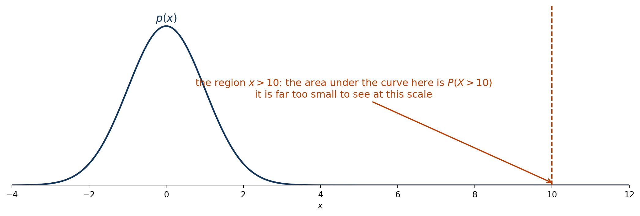
Let \(X \sim \mathcal{N}(0,1)\), with density \(p(x) = \frac{1}{\sqrt{2\pi}} e^{-x^2/2}\). Estimate \(P(X > 10)\).

\[ P(X > 10) = \int \mathbb{1}[x > 10] \, p(x) \, dx = \mathbb{E}_p\big[\mathbb{1}[X > 10]\big] \]

That is an expectation of the indicator \(h(x) = \mathbb{1}[x > 10]\) under \(p\), so Monte Carlo applies.

Task 6: try the obvious thing

# TODO: draw 10 million standard normals and compute the fraction above 10
naive = ...
print(naive)

Why is it zero?

• How many of your ten million samples are greater than \(10\)?
• How many samples would you need to draw to get one sample greater than \(10\), in expectation?
• Is the estimator biased?

Importance sampling

Sample from somewhere useful instead, and correct for it. For a target density \(p\) and any density \(q\) with \(q(x) > 0\) wherever \(h(x)\,p(x) \neq 0\):

\[ \begin{aligned} \mathbb{E}_p[h(X)] &= \int h(x)\, p(x)\, dx \\ &= \int h(x)\, p(x)\, \frac{q(x)}{q(x)}\, dx \\ &= \int h(x)\, \frac{p(x)}{q(x)}\, q(x)\, dx \\ &= \mathbb{E}_q\!\left[ h(X)\, w(X) \right], \qquad w(x) = \frac{p(x)}{q(x)}. \end{aligned} \]

• Draw \(x_k \sim q\), the proposal, chosen to put mass where \(h\,p\) is nonzero.
• Weight each draw by \(w(x_k)\) to undo the change of distribution.
• The estimator \(\frac{1}{K}\sum_k h(x_k)\, w(x_k)\) is unbiased for any \(q\) satisfying the support condition above. Only the variance changes.

Task 7: the estimator

x0 = 10
# TODO: sample 100,000 draws from N(x0, 1)
# TODO: compute weights = p(x)/q(x) using ss.norm.pdf twice (target, then proposal)
# TODO: estimate as the mean of weights * (x > x0)
assert abs(estimate - ss.norm.sf(x0)) / ss.norm.sf(x0) < 0.05

A hundred thousand samples from the right place beat ten million from the wrong one.

Task 8: does the proposal matter?

# Compare three proposals, all with num_samples = 10,000:
#   (a) N(10, 1)
#   (b) N(10, 2)
#   (c) 10 + Exponential(1)      <- check how scipy.stats parameterizes the exponential
# For each, report the estimate and the relative standard error
#       v = weights * (x > x0);   v.std() / v.mean() / sqrt(num_samples)

All three are unbiased. They are not equally good, and the ranking may surprise you – think about which proposal has tails shaped most like the integrand.

What makes a proposal good

Important

The variance of the weights is everything. If \(q\) has lighter tails than \(p\), some \(w(x) = p/q\) become enormous, a handful of samples dominate the average, and the estimator is unusable while still looking fine.

• Rule of thumb: the proposal should be at least as heavy tailed as the target.
• Diagnostic: look at the largest few weights. If one sample carries most of the total weight, you are in trouble.
• This is the central difficulty of sequential Monte Carlo later in the course, where the weights degenerate over time.

Wrapping up

What to submit

A rendered lab2.qmd (.qmd and .html) containing:

1. Task 1 with its plot.
2. Tasks 2 and 3: the Monte Carlo estimate and the conjugacy check agreeing.
3. Task 4’s log-log plot, with a sentence on the slope.
4. Task 5: the log space estimator, matching the closed form.
5. Tasks 6-8: the naive attempt, the importance sampling estimator, and your comparison of the three proposals.

Due at the start of next week’s lab.

Checklist

• Task 2 gives about \(1.24 \times 10^{-25}\)
• exact_marginal(0.5) and exact_marginal(0.31) return the same number
• Task 5 gives about \(-57.34\), matching betaln(s+1, N-s+1)
• Task 7 is within 5% of ss.norm.sf(10)
• every random draw comes from a seeded default_rng

Task 3 evaluated \(p(y) = p(y \mid \theta)p(\theta) / p(\theta \mid y)\) at an arbitrary \(\theta\) and got the exact answer with no integration at all. Why can we not always do this, and what did conjugacy actually buy us?