from scipy.stats import multivariate_normalfrom scipy.special import logsumexpX = X_geyser[:5] # 5 rows, D = 2mu, Sigma = X.mean(axis=0), np.cov(X, rowvar=False)r = np.array([[0.9, 0.1], [0.2, 0.8], [0.5, 0.5], [1.0, 0.0], [0.3, 0.7]])# 1. log density of every row under one Gaussian, in one callprint(multivariate_normal(mu, Sigma).logpdf(X).round(2))# 2. one column per component, stacked into an (N, K) matrixmus = [mu -1, mu +1] # two made-up componentsL = np.column_stack([multivariate_normal(mus[k], Sigma).logpdf(X) for k inrange(2)])print(L.shape)# 3. normalize rows on the log scale# [:, None] turns a length-N vector into an (N, 1) column, so subtracting it# takes each row's own value off that rowprint(np.exp(L - logsumexp(L, axis=1)[:, None]).sum(axis=1))# 4. weighted sums of rows: r.T @ X gives a (K, D) matrix of sum_i r_ik y_iprint((r.T @ X) / r.sum(axis=0)[:, None])# 5. a dict bundles named results; build it with dict(...), read it with ["name"]fit =dict(mu=mu, Sigma=Sigma, ll=-1130.3)print(fit["ll"], fit["mu"].shape)
def init(X, K, rng):""" Returns mu (K, D), Sigma (K, D, D), pi (K,) """# TODO: mu = K distinct rows of X, chosen with rng.choice(..., replace=False)# TODO: Sigma = the pooled covariance np.cov(X, rowvar=False), one copy per component# TODO: pi = 1/K for every componentraiseNotImplementedError
Use exactly this recipe. The lecture did, and your numbers are expected to match its numbers.
Task 2: the E-step
def e_step(X, mu, Sigma, pi):""" X : (N, D) data mu : (K, D) means Sigma : (K, D, D) covariances pi : (K,) mixing weights Returns ------- r : (N, K) responsibilities, rows summing to 1 ll : scalar, the observed data log likelihood at these parameters """# TODO# 1. log_r: the (N, K) matrix of log pi_k + log N(y_i; mu_k, Sigma_k)# 2. ll_i = logsumexp over k -> this is log p(y_i | theta); ll is its sum# 3. r = exp(log_r - ll_i[:, None])raiseNotImplementedError
Important
Work on the log scale and normalize with logsumexp. The logsumexp of each row is \(\log p(y_i \mid \theta)\), so the E-step hands you the objective for free.
Task 3: the M-step
def m_step(X, r, reg=1e-6):""" X : (N, D) r : (N, K) responsibilities from the E-step Returns mu (K, D), Sigma (K, D, D), pi (K,) """# TODO# N_k = column sums of r# mu_k = weighted mean (idiom 4)# Sigma_k = weighted covariance, using the NEW mu_k, then add reg * I# pi_k = N_k / NraiseNotImplementedError
One hint: (r[:, [k]] * (X - mu[k])).T @ (X - mu[k]) is the weighted scatter matrix for component \(k\).
Task 4: the loop
def em_gmm(X, K, seed=0, max_iter=500, tol=1e-6, reg=1e-6):""" Returns a dict with keys mu, Sigma, pi, r, trace, iters, ll. r is the (N, K) responsibility matrix at the final parameters; trace is the list of log likelihoods, one per iteration. """ rng = np.random.default_rng(seed) mu, Sigma, pi = init(X, K, rng) trace = []# TODO: for t in range(max_iter):# r, ll = e_step(...) -> append ll to trace# mu, Sigma, pi = m_step(...)# stop when t > 0 and the change in ll is below tol# TODO: one last e_step at the final parameters, so r and ll match mu, Sigma, pi# TODO: return dict(mu=mu, Sigma=Sigma, pi=pi, r=r, trace=trace, iters=t + 1, ll=ll)raiseNotImplementedError
Follow this order exactly: record \(\ell\)before each M-step, and finish with an E-step. The figures need responsibilities that belong to the parameters you return.
Task 5: check the theory
Wednesday’s derivation says the observed data log likelihood can never decrease. Verify it:
fit = em_gmm(X_geyser, K=2, seed=0)diffs = np.diff(fit["trace"])assert np.all(diffs >=-1e-8), "log likelihood decreased -- there is a bug"print(f"monotone over {len(diffs)} iterations, final ll = {fit['ll']:.1f}")plt.plot(fit["trace"], marker="o", markersize=3)plt.xlabel("iteration"); plt.ylabel(r"$\ell(\theta)$"); plt.show()
Note
This assertion is the most useful debugging tool you have. If it fails, the bug is almost always in the M-step: a wrong denominator, or the old\(\mu_k\) inside the covariance update.
Task 6: restarts
Random initialization can land in a local optimum. Run several seeds and keep the best:
def best_of(X, K, seeds=range(10), reg=1e-6):"""Run em_gmm once per seed, passing reg through, and return the fit with the highest ll."""# TODOraiseNotImplementedError
best_of must return the same dict as em_gmm. Everything from here on is built from that dict.
Helpers you may use as given
Cluster labels are arbitrary, so before scoring a fit its labels are permuted to line up with the recorded ones. These three functions are the lecture’s, unchanged.
from itertools import permutationsfrom matplotlib.patches import Ellipsedef align(codes, pred, K):"""Permute predicted labels to agree as much as possible with the true codes.""" best =max(permutations(range(K)), key=lambda q: (np.array(q)[pred] == codes).mean())return np.array(best)[pred]def draw_ellipse(ax, mu, Sigma, n_std=2): vals, vecs = np.linalg.eigh(Sigma) order = vals.argsort()[::-1] vals, vecs = vals[order], vecs[:, order] angle = np.degrees(np.arctan2(vecs[1, 0], vecs[0, 0])) ax.add_patch(Ellipse(mu, *(2* n_std * np.sqrt(vals)), angle=angle, fc="none", ec="black", lw=2.5))def compare(X, fit, truth, xlab, ylab):"""Two panels: recorded labels, and EM clusters with 2 sd ellipses. Returns the agreement.""" cat = pd.Categorical(truth) pred = align(cat.codes, fit["r"].argmax(axis=1), len(fit["pi"])) fig, axes = plt.subplots(1, 2, figsize=(14, 5))for ax, lab, title in [(axes[0], cat, "true labels"), (axes[1], cat.categories[pred], "EM clusters")]: sns.scatterplot(x=X[:, 0], y=X[:, 1], hue=np.asarray(lab), ax=ax, s=25, hue_order=list(cat.categories)) ax.set_title(title); ax.set_xlabel(xlab); ax.set_ylabel(ylab)for k inrange(len(fit["pi"])): draw_ellipse(axes[1], fit["mu"][k], fit["Sigma"][k]) plt.tight_layout(); plt.show()return (pred == cat.codes).mean()
Read compare once: it uses fit["r"], fit["mu"], fit["Sigma"] and fit["pi"]. That is why Task 4 returns them.
Task 7: Old Faithful
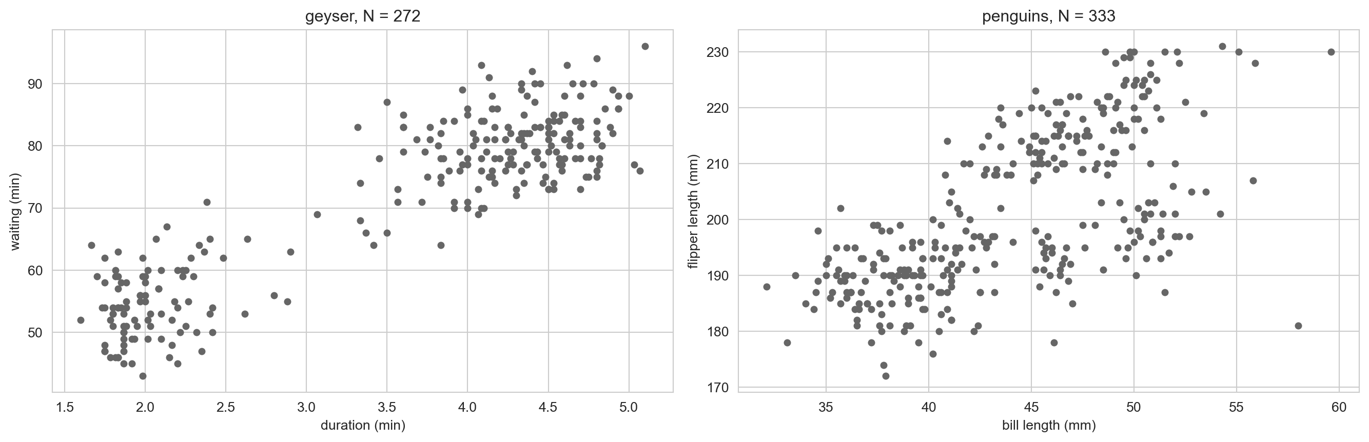
Fit two components and reproduce the lecture’s figure:
fit_geyser = best_of(X_geyser, K=2)print(f"converged in {fit_geyser['iters']} iterations, log lik = {fit_geyser['ll']:.1f}")print(f"pi = {np.round(fit_geyser['pi'], 2)}")print(f"mu = {np.round(fit_geyser['mu'], 1).tolist()}")# TODO: print each Sigma_k, rounded to one decimalacc = compare(X_geyser, fit_geyser, faithful["kind"].to_numpy(), "duration (min)", "waiting (min)")print(f"agreement with the recorded kind: {acc:.1%}")
Targets from the lecture: log likelihood \(-1130.3\), \(\pi \approx (0.36, 0.64)\), agreement \(98.2\%\). If you are far off, go back to Task 5.
Task 8: Penguins
Fit three components with only the two measurements above:
fit_peng = best_of(X_peng, K=3)# TODO: the same report as Task 7, thenacc = compare(X_peng, fit_peng, penguins["species"].to_numpy(), "bill length (mm)", "flipper length (mm)")print(f"agreement with species: {acc:.1%}")# TODO: the confusion table. Align the labels first:codes = pd.Categorical(penguins["species"]).codescategories = pd.Categorical(penguins["species"]).categoriespred = align(codes, fit_peng["r"].argmax(axis=1), 3)pd.crosstab(penguins["species"].to_numpy(), categories[pred], rownames=["true"], colnames=["EM"])
Targets: log likelihood \(-2187.6\), agreement \(94.6\%\). The errors should sit on the Adelie/Chinstrap boundary, as in the lecture.
Task 9: restarts are not optional
Run the ten seeds on the penguins one at a time and tabulate them:
rows = []for s inrange(10): f = em_gmm(X_peng, 3, seed=s)# TODO: append a dict with seed, log lik (1 decimal), iterations,# and agreement with species after aligning labelspd.DataFrame(rows)
At least one seed lands in a worse optimum. Report which, and by how much its log likelihood and agreement fall short. Write:best_of picked the good fit without seeing a single label. What did it use instead?
Task 10: generate from the fit
A fitted mixture is a generative model. Run it forwards:
rng = np.random.default_rng(1)# TODO: z_new = rng.choice(3, size=N, p=fit_peng["pi"])# TODO: one draw from multivariate_normal(mu[z], Sigma[z]) for each z in z_new -> (N, 2) array Y_newfig, axes = plt.subplots(1, 2, figsize=(14, 5), sharex=True, sharey=True)axes[0].scatter(X_peng[:, 0], X_peng[:, 1], s=20, color="0.4"); axes[0].set_title("observed penguins")axes[1].scatter(Y_new[:, 0], Y_new[:, 1], s=20, c=z_new, cmap="Set2"); axes[1].set_title("simulated from the fit")for ax in axes: ax.set_xlabel("bill length (mm)")axes[0].set_ylabel("flipper length (mm)")plt.tight_layout(); plt.show()
Write: one sentence on where the simulated data look like the real data and one on where they do not.
Task 11: three experiments
Short experiments, one or two sentences of explanation each.
All four measurements, and a collapse. Refit the penguins with bill_length_mm, bill_depth_mm, flipper_length_mm, body_mass_g, running the ten seeds one at a time. One seed raises LinAlgError: a component has collapsed onto a few points and its \(\Sigma_k\) is no longer positive definite. Print that component’s soft count \(N_k\) and the eigenvalues of its \(\Sigma_k\) on the iteration before the failure. Then explain why reg = 1e-6 did nothing here (look at the scale of body_mass_g), fix it, and report the agreement of the best surviving fit. Which pair of species stopped being confused?
Monday’s homework, numerically. Start em_gmm from \(r_{ik} = 1/K\) instead of Task 1’s initialization, by calling m_step first. Print the parameters the first M-step returns and the responsibilities the next E-step returns. Does the algorithm ever recover?
Where is the underflow? Replace the logsumexp normalization with a direct division of multivariate_normal.pdf values and rerun Task 8. Does anything break? Find the smallest entry of your log_r matrix in the best fit and estimate how many independent measurements like these it would take before exp returns zero for a whole row. (float64 underflows below about \(e^{-745}\).)
Task 12 (stretch): how many components, and a reference check
You were told \(K\). Fit \(K = 1, \ldots, 6\) to the penguins and plot
\[
\text{BIC} = -2 \, \ell(\hat{\theta}) + P \log N, \qquad P = (K-1) + KD + K \tfrac{D(D+1)}{2}.
\]
Does the minimum land on three? If it does not, look at the fit BIC prefers and say what the extra component is doing.
from sklearn.mixture import GaussianMixtureref = GaussianMixture(3, covariance_type="full", n_init=10, random_state=0).fit(X_peng)print(ref.score(X_peng) * X_peng.shape[0]) # sklearn reports the mean; multiply by N
Your log likelihood should match to within a fraction of a nat. If yours is higher, you have not made an error. You may simply have found a better optimum.