Department of Biostatistics and Computational Biology, University of Rochester Medical Center
Where we left off
Forward-backward turned a sum over \(K^T\) state paths into \(O(TK^2)\) work by pushing each sum as far inward as it would go.
What that used: the joint factorized into terms that each touch two neighbouring variables; every partial sum could be computed once and reused.
Nothing in the argument was about time. The chain is just the simplest arrangement with that property.
The next simplest is a tree, and the same two passes work there. The algorithm is called belief propagation.
In Lab 4 you built the data structure, wrote the two traversals, and simulated an alignment down a phylogeny. Today we hang the inference on that code, then apply it to compute a likelihood of a phylogeny.
Goals
State what a tree structured model assumes, and why that assumption lets sums be pushed inward.
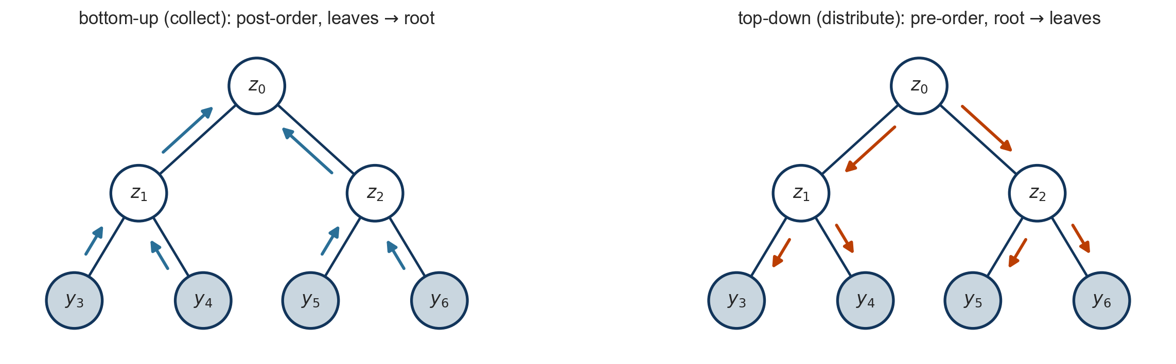
Derive the message rule and the bottom-up (collect) and top-down (distribute) passes by pushing sums inward on a small tree.
Relate belief propagation on a tree to forward-backward on a chain.
Recognize Felsenstein’s pruning algorithm as the bottom-up pass, use it to score phylogenies, and use the top-down pass to infer ancestral states.
Tree structured models
Trees
An undirected graph is a tree if it is connected and has no cycles. Equivalently:
There is exactly one path between any two nodes.
\(n\) nodes, \(n - 1\) edges.
Removing any edge splits the graph into two pieces.
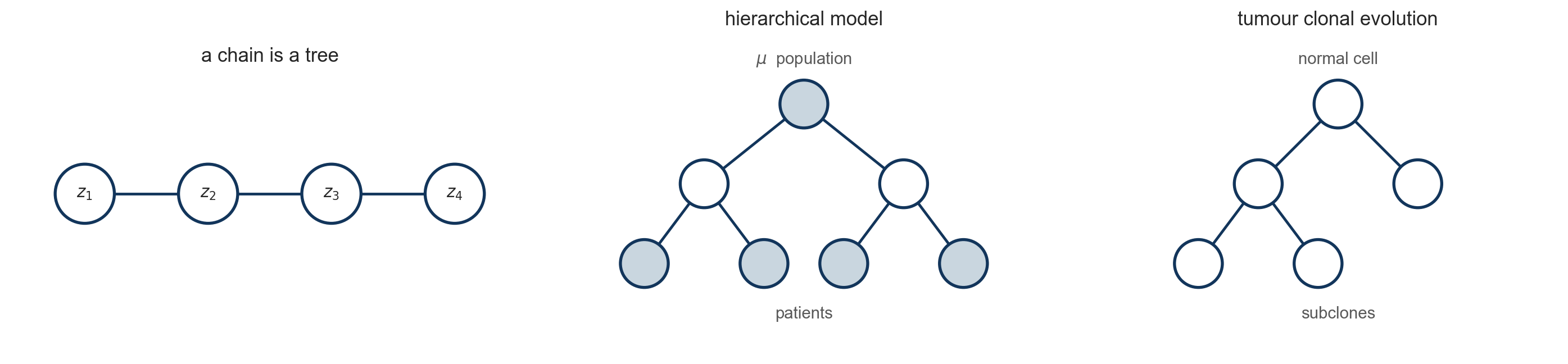
A tree structured model is a joint distribution whose factors each involve one node or one edge of some tree. The HMM is one: its factors are \(p(z_t \mid z_{t-1})\) on the edges and \(p(y_t \mid z_t)\) at the nodes, and the tree is a line.
A latent tree model
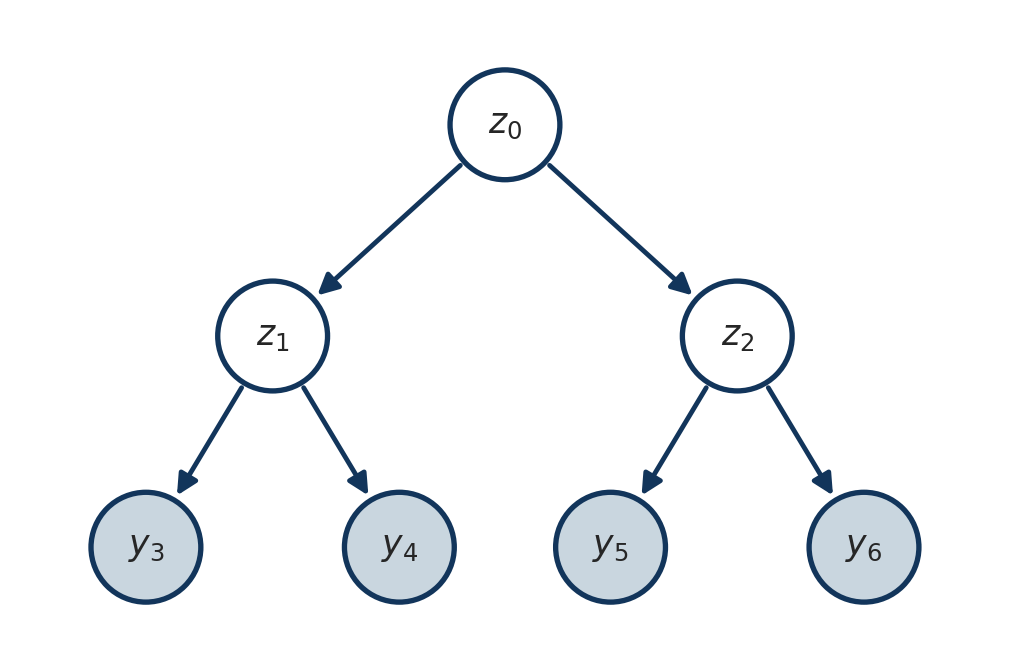
Latent variables at the internal nodes, observations at the leaves. The HMM had one observation hanging off each latent variable; here the shape is richer, but the factorization is the same kind of object.
Exercise. Write down the joint distribution \(p(\mathbf{z}, \mathbf{y})\) of this model by following the arrows: one factor per node, conditioned on whatever points at it. How many terms does the likelihood \(p(\mathbf{y})\) sum over if each \(z\) takes \(K\) values?
The joint distribution
For a uniform message-passing notation, place a state \(z_v\) at every node and attach data through \(p(y_v \mid z_v)\). At an observed leaf, deterministic observation makes this equivalent to the collapsed picture on the previous slide.
Write \(\mathbf{z} = (z_1, \ldots, z_n)\) for the latent variables at the \(n\) nodes, one multivariate variable, and \(\mathbf{y}\) for the observations. For a directed tree with root \(r\), the chain rule along the arrows gives
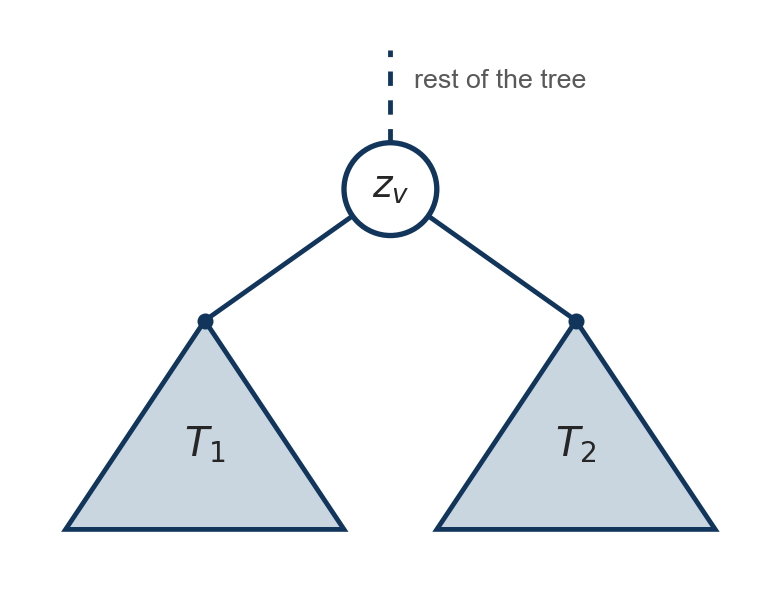
Once \(z_v\) is fixed, no term in the joint distribution involves variables from both \(T_1\) and \(T_2\). The only path between the two subtrees runs through \(v\), so the joint distribution separates into one part for each subtree.
So a sum over \(T_1\) and a sum over \(T_2\) can be done separately and multiplied. That is the conditional independence we used on the chain, where \(z_t\) separated the past from the future.
With a cycle there would be two routes between some pair of variables, one node would not separate them, and the sums would not split.
The same problem as before
The likelihood of the leaves sums the joint over every latent node:
\(K^n\) terms, where \(n\) is now the number of internal nodes rather than the length of a sequence.
Same disease, same cure. Push the sums inward.
Trees are not an exotic special case
Phylogenies and clonal trees, from the lab: species, viral lineages, B cell receptors, tumour subclones. Ancestors at the internal nodes, sequenced data at the leaves. The second half of today.
Hierarchical models. Patients within clinics within regions. The latent variables are the group level parameters, and observing one clinic tells you about the others only through their shared parent. Same shape, no evolution.
Hierarchical labels. A taxonomy of diagnoses or cell types, where a label at a leaf implies every ancestor label.
Pushing sums inward
A small tree, written out
Four leaves, three latent nodes, states in \(\{1, \dots, K\}\). Nothing is observed at the latent nodes themselves.
Each bracket depends only on \(z_0\) and only on the subtree below one child. Three sums of \(K^2\) terms instead of one sum of \(K^3\).
A quantity for every subtree
Inside the first bracket, \(p(y_3 \mid z_1)\) is itself a function of \(z_1\) alone, “what leaf 3 says about \(z_1\)”. Call it \(m_{3 \to 1}(z_1)\). Then the bracket is
A message is a likelihood: what the data below \(v\) say about the state at the far end of the edge. On the small tree, \(m_{1 \to 0}(z_0) = p(y_3, y_4 \mid z_0)\).
On the chain this was \(\beta_t(k) = p(y_{t+1:T} \mid z_t = k)\). Same object, read on a tree.
Exercise. Prove the two identities above by induction from the leaves to the root. For the inductive step, condition on \(z_v\), use the independence of its child subtrees, and then sum over \(z_v\).
The bottom-up (collect) pass
Run the rule once per non-root node, children before parents. At the root nothing is left to send, so sum instead:
One message per edge, each a sum over \(K\) values for each of \(K\) outputs: \(O(K^2)\) per edge, \(O(nK^2)\) in all.
The root’s subtree is the whole tree, so the final step multiplies the likelihood given the root state by its prior and sums over that state.
This is the whole likelihood computation. For the phylogenetics half of today it is the only pass we need.
Marginals need the other direction
The posterior at an internal node \(v\) is the joint with everything except \(z_v\) summed out. Everything below \(v\) is already in hand. What is missing is everything above:
\[
p(z_v, \mathbf{y}) \;=\; \underbrace{p(\mathbf{y}_{\lceil v \rceil}, z_v)}_{\text{from the parent } u} \; \underbrace{p(y_v \mid z_v) \prod_{c \,\in\, \text{children}(v)} m_{c \to v}(z_v)}_{p(\mathbf{y}_{\lfloor v \rfloor} \mid z_v), \text{ from the children of } v}
\]
Write \(\mathbf{y}_{\lceil v \rceil} := \mathbf{y} \setminus \mathbf{y}_{\lfloor v \rfloor}\) for the complement: every observation not in the subtree at \(v\). Given \(z_v\) the two sides are independent, so the joint factorizes as shown, and \(p(z_v \mid \mathbf{y})\) is this divided by \(p(\mathbf{y})\).
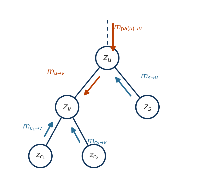
The subtree likelihood \(p(\mathbf{y}_{\lfloor v \rfloor} \mid z_v)\) is available after the bottom-up pass. The missing term is \(m_{u \to v}(z_v) := p(\mathbf{y}_{\lceil v \rceil}, z_v)\): the data outside \(v\)’s subtree, jointly with \(z_v\).
The top-down message
“Above \(v\)” is the rest of the tree once the edge \((u, v)\) is cut. Seen from \(u\), that is three things, all functions of \(z_u\): \(u\)’s own evidence, whatever came down to \(u\) from its parent, and the subtrees of \(v\)’s siblings. Multiply them, attach the edge, and sum out \(z_u\):
\[
\boxed{\; m_{u \to v}(z_v) = \sum_{z_u} p(z_v \mid z_u) \, \underbrace{p(y_u \mid z_u)}_{\text{evidence at } u} \, \underbrace{m_{\text{pa}(u) \to u}(z_u)}_{\text{from above } u} \underbrace{\prod_{s \,\in\, \text{children}(u),\; s \neq v} m_{s \to u}(z_u)}_{\text{from the siblings of } v} \;}
\]
At the root nothing is above, \(\mathbf{y}_{\lceil r \rceil}\) is empty, and \(p(\mathbf{y}_{\lceil r \rceil}, z_r) = p(z_r)\): the prior is what the root “hears from above”. Set \(m_{\text{pa}(r) \to r}(z_r) := p(z_r)\).
A node’s top-down message needs its parent’s first: pre-order, the mirror image of the bottom-up pass.
One rule
Write \(\mathcal{N}(i)\) for the neighbours of \(i\), parent and children alike. Both boxed formulas are the same statement:
where \((\text{pa}, \text{ch})\) is the edge \(\{i, j\}\) read in the direction of its arrow, and the root’s prior counts as a message arriving from above.
Take everything \(i\) knows, its own evidence and every incoming message except the one from \(j\), multiply, attach the edge, sum out \(z_i\).
Excluding \(j\)’s message is what keeps the subtree on \(j\)’s side from being counted twice. On a tree the two sides of an edge share nothing else, so this is exactly right.
Parent or child, up or down: one rule, applied once per edge per direction.
The schedule
Pick any node as root. Pass messages bottom-up, then top-down. Each edge carries one message in each direction: \(2(n - 1)\) messages at \(O(K^2)\) apiece, and then every marginal in the model is a product of vectors.
Exercise: it really is the marginal
Throughout, \(v\) is a node and \(u = \text{pa}(v)\) is its parent, so \(m_{v \to u}\) travels up and \(m_{u \to v}\) travels down. Everything needed is the factorization of \(p(\mathbf{z}, \mathbf{y})\) and the separation property, used once per step.
Bottom-up. Show by induction from the leaves that \(m_{v \to u}(z_u) = p(\mathbf{y}_{\lfloor v \rfloor} \mid z_u)\). The leaf case is one line; for an internal node use that, given \(z_v\), the children’s subtrees are independent of each other.
Top-down. Show that \(m_{u \to v}(z_v) = p(\mathbf{y}_{\lceil v \rceil}, z_v)\), by induction from the root, where \(\mathbf{y}_{\lceil v \rceil} = \mathbf{y} \setminus \mathbf{y}_{\lfloor v \rfloor}\). First check that removing the subtree at \(v\) leaves three pieces, the complement of \(u\)’s subtree, \(u\)’s own observation, and the subtrees of \(u\)’s other children, \[
\mathbf{y}_{\lceil v \rceil} = \mathbf{y}_{\lceil u \rceil} \;\cup\; \{y_u\} \;\cup \bigcup_{s \,\in\, \text{children}(u) \setminus \{v\}} \mathbf{y}_{\lfloor s \rfloor},
\] and that the three are independent given \(z_u\).
Together. Conclude that \(p(y_v \mid z_v) \prod_c m_{c \to v}(z_v) \, m_{u \to v}(z_v) = p(z_v, \mathbf{y})\) at every node, so that summing it over \(z_v\) gives \(p(\mathbf{y})\) at every node, not only at the root. On the chain this was \(\sum_k \alpha_t(k) \beta_t(k) = p(y_{1:T})\) for every \(t\).
Edges. Write \(p(z_u, z_v, \mathbf{y})\) for the edge from \(u\) down to \(v\) as a product of messages, the edge conditional \(p(z_v \mid z_u)\), and evidence. Dividing by \(p(\mathbf{y})\) gives the edge posterior \(p(z_u, z_v \mid \mathbf{y})\), the tree analogue of \(\xi_t(i,j) = p(z_{t-1}=i, z_t=j \mid y_{1:T})\) in an HMM.
Phylogenetics
The oldest tree model in biology
Evolutionary biology. Which species are most closely related, and in what order did they diverge?
Molecular epidemiology. SARS-CoV-2 lineages, influenza strain selection, tracing an outbreak to its source. A phylogeny of viral genomes is a transmission history.
Cancer genomics. Subclones are related by descent; the clonal tree is the order in which driver mutations were acquired.
Immunology. B cell receptor lineages in a germinal centre are a phylogeny of somatic hypermutation.
In every case the ancestors are unobserved. That is what makes it a latent variable problem, and its inference algorithm, published in 1981, is exactly the bottom-up pass we just derived.
The data
tree = build_tree()rng = np.random.default_rng(5)simulate_sites(tree, n_sites=300, rng=rng)by_name = {v.name: v for v in preorder(tree)}for name in"ABCD":print(f"{name}{to_string(by_name[name].seq[:48])} ...")
A  GTATCTCCTAACGCAAAAATAGTGCGCTACATACGCGGGATGTCCTAA ...
B  GTAACCACTACTGCCTTAACGATTCGCTACATACGCGGCATGTCCTAA ...
C  GCAACGGTTACCGGATAAAAACTACCCGGTTTAGCAGGGGGGGTCTAA ...
D  GTATCGGCTACCGCATAAATACTTCCCAATTGAGCACGTATGATCTAA ...
The alignment you simulated in Lab 4: one row per taxon, one column per site, and three ancestral rows we now pretend not to have.
Given the tree, sites are assumed independent, so the likelihood is a product over columns and everything can be developed for one column at a time.
Real alignments have \(10^3\) to \(10^6\) columns. The leaves are data; the tree and the ancestors are the unknowns.
The tree is two unknowns
Topology: who is related to whom. Discrete, and the number of them is enormous.
Branch lengths\(t_e\): expected substitutions per site along each branch. Continuous, one per edge.
Both must usually be inferred. The ancestral nucleotides at the internal nodes are latent variables, \(K = 4\), one per node per site.
Rooted or unrooted? Most substitution models are time reversible, so the likelihood comes out the same wherever the root is placed. We pick a root anyway, because the traversals need a starting point and because a rooted tree reads as a history.
How many topologies?
taxa
unrooted topologies
4
3
5
15
10
2.027e+06
20
2.216e+20
50
2.838e+74
Fifty taxa, a small study, gives \(10^{74}\) topologies. The tree can no more be found by enumeration than the state path could. Every search strategy relies on scoring a candidate tree fast, and that is what the rest of today buys.
Substitution along a branch
A site evolves along a branch as a continuous time Markov chain on \(\{A, C, G, T\}\) with rate matrix \(Q\), so the transition matrix for a branch of length \(t\) is \(P(t) = e^{Qt}\), with
\(P(s)P(t) = P(s + t)\): the model is consistent however a branch is subdivided.
Under Jukes-Cantor, \(P(t)\) is the closed form you used to simulate. K80 separates transitions from transversions; GTR has six exchangeabilities and four base frequencies; a Gamma distributed rate per site lets some columns evolve faster than others.
None of that changes what follows. The algorithm needs only a matrix \(P(t)\) per branch and a root distribution \(\pi\); swap the model and the inference code is untouched.
Three internal nodes, \(4^3 = 64\) terms. Fifty taxa gives \(4^{49} \approx 3 \times 10^{29}\), per site, with thousands of sites, repeated for every candidate tree.
It is the tree model, with every node carrying a nucleotide \(z_v\): \(p(z_{\text{root}}) = \pi\) and \(p(z_v \mid z_{\text{pa}(v)}) = P(t_v)\). Nothing is observed at an internal node, so its evidence factor is absent. At a leaf the nucleotide itself is observed, \(y_v = z_v\), so the evidence is the indicator \(p(y_v \mid z_v) = \mathbb{1}[z_v = y_v]\).
So we already know the way out.
Felsenstein’s pruning algorithm
Define the conditional likelihood of the subtree below \(v\), given that \(v\) is in state \(s\):
One post-order traversal. \(O(nK^2)\) instead of \(O(K^n)\).
Exercise: pruning is message passing
Let \(v\) be an internal node in state \(s\), with children \(c\). Starting from the bottom-up message rule:
Nothing is observed at an internal node, so its evidence factor is absent. At a leaf the latent state is the observed nucleotide itself, so the factor is \(\mathbb{1}[z_v = y_v]\). Say why these two conventions make the leaf rule \(L_v(s) = \mathbb{1}[s = y_v]\) the bottom-up message rule with no children.
If the conditional likelihood below child \(c\) is \(L_c(s')\), show that \[
m_{c \to v}(s)=\sum_{s'} P_{ss'}(t_c)L_c(s').
\]
Multiply the child messages and recover the internal-node pruning rule \[
L_v(s)=\prod_c m_{c \to v}(s).
\]
\(\mathbb{1}[s=y_v]\) at a leaf, \(1\) at an internal node
conditional \(p(z_v \mid z_{\text{pa}(v)})\)
transition matrix \(P(t_v)\)
\(p(\mathbf{y})\) at the root
\(\sum_s \pi_s L_{\text{root}}(s)\)
Felsenstein published this in 1981; Pearl’s belief propagation came in 1982. Two communities derived the same algorithm within a year of each other, and it took a decade for anyone to notice.
Exercise: one column by hand
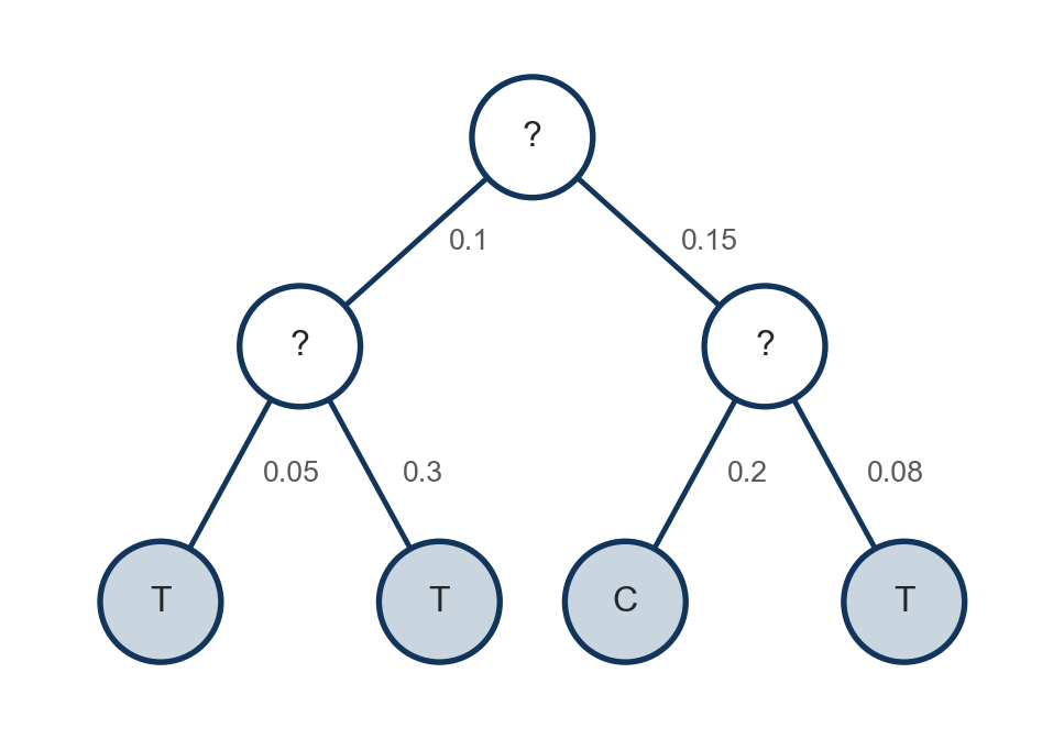
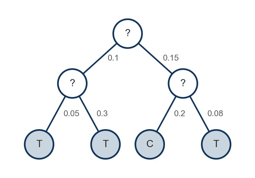
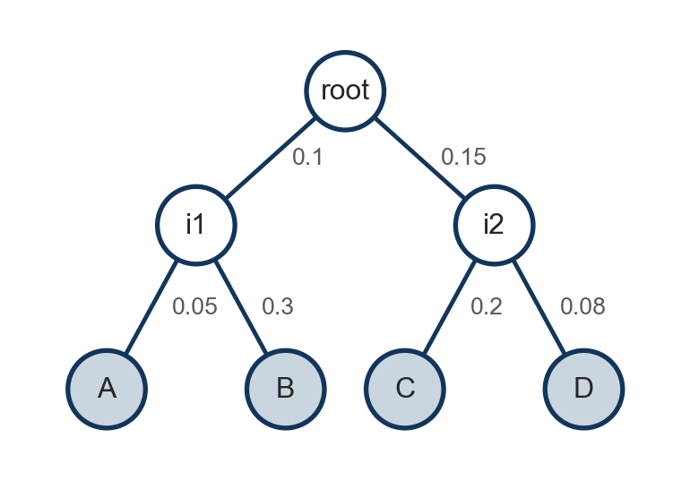
Column \(s\) of the alignment is \(\mathbf{y}^{(s)} = (y_A, y_B, y_C, y_D)\), shown at the leaves, with the branch lengths on the branches. Marginalize out the three ancestors.
Write \(p(\mathbf{y}^{(s)} \mid \tau, \mathbf{t})\) as a sum over \(z_{\text{root}}, z_{i_1}, z_{i_2}\): \(64\) terms, each a product of \(\pi\) and five entries of Jukes-Cantor matrices.
Push each sum as far inward as it goes. You should arrive at \(L_{i_1}\), \(L_{i_2}\) and \(L_{\text{root}}\) as vectors of length four. Compute them with jc69, and finish with \(\sum_a \pi_a L_{\text{root}}(a)\).
Add up all \(64\) terms directly and check that the two numbers agree.
for the record, column 1 is TTCT and p(y^(s)) = 7.938823e-03
A whole alignment
A  GTATCTCCTAACGCAAAAATAGTGCGCTACATACGC ...
B  GTAACCACTACTGCCTTAACGATTCGCTACATACGC ...
C  GCAACGGTTACCGGATAAAAACTACCCGGTTTAGCA ...
D  GTATCGGCTACCGCATAAATACTTCCCAATTGAGCA ...

   300 columns
Sites are assumed independent given the tree, so the log likelihood of the alignment is the sum of the column log likelihoods, each one a bottom-up pass on this tree with these branch lengths.
set_site: evidence and transition matrices for one column; alignment_loglik: the sum over columns
def set_site(root, site, pi=np.full(4, 0.25)):for v in preorder(root):if v.is_leaf(): v.pot = np.zeros(4); v.pot[v.seq[site]] =1.0# the leaf's nucleotide is observed: a point masselse: v.pot = np.ones(4) # nothing observed at an internal nodeif v.parent isnotNone: v.edge = jc69(v.branch_length) # p(z_v | z_pa) = P(t_v) root.pot = root.pot * pi # the prior, folded into the rootdef site_likelihood(root, site): set_site(root, site)return collect(root)def alignment_loglik(root, n_sites):returnsum(np.log(site_likelihood(root, s)) for s inrange(n_sites))print(f"log p(y | tau, t) = {alignment_loglik(tree, 300):.2f}")
log p(y | tau, t) = -1222.80
Three hundred columns, six messages each, every one a \(4 \times 4\) matrix times a vector. A real package vectorizes over columns and scores a million of them in well under a second.
The number depends on the topology \(\tau\) and on the branch lengths \(\mathbf{t}\). Vary one, then the other.
How much do the branch lengths matter?
Scale every branch length by a common factor and score the alignment again. The data were simulated at factor \(1\).
factor
log likelihood
0.25
-1367.8
0.5
-1269.4
1.0
-1222.8
2.0
-1266.8
4.0
-1430.0
Too short and every difference between leaves is nearly impossible; too long and every column looks like four independent draws from \(\pi\), which is improbable when the leaves mostly agree. The likelihood is highest near the lengths that generated the data, and with a real alignment this is how branch lengths are estimated.
With every branch scaled together this is a one dimensional search. Real software optimizes each branch length separately, calling the bottom-up pass inside the optimizer.
Choosing between trees
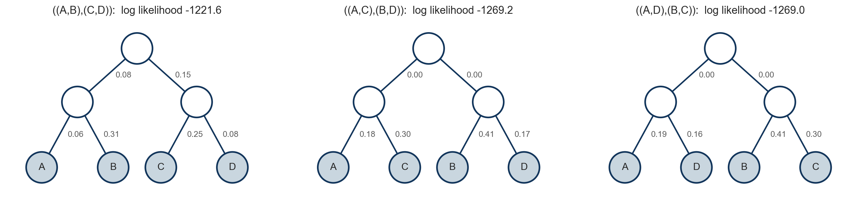
Four taxa admit three unrooted topologies. Score each on the same leaf rows.
Each tree is shown with its own maximum likelihood branch lengths, fitted one branch at a time with the bottom-up pass inside the optimizer. The true topology recovers lengths close to the ones that generated the data. The wrong ones do the only thing they can: shrink the internal branches to zero, which turns both into the same star tree with the same likelihood, nearly fifty log units behind.
Scoring a tree is cheap. Finding the right one among \(10^{74}\) is the problem.
Ancestral states: one column
The top-down pass gives, for every internal node \(v\) and column \(s\), the posterior over its nucleotide given that column:
\[
p(z_v^{(s)} \mid \mathbf{y}^{(s)}) = \frac{p(\mathbf{y}_{\lceil v \rceil}^{(s)}, z_v^{(s)}) \; p(\mathbf{y}_{\lfloor v \rfloor}^{(s)} \mid z_v^{(s)})}{p(\mathbf{y}^{(s)})}.
\]
node \(v\)
A
C
G
T
argmax
truth
root
0.004
0.015
0.004
0.978
T
T
i1
0.000
0.001
0.000
0.999
T
T
i2
0.002
0.034
0.002
0.961
T
T
The column is the one from the exercise on slide 31, T T C T. Each row is \(p(z_v^{(s)} \mid \mathbf{y}^{(s)})\) over the four nucleotides; the largest entry is the posterior mode for that node, one node at a time.
i2 sees C from one child and T from the other, yet lands on T with probability \(0.96\). Three things combine. From below, D says T along a short branch, where a change is unlikely, while C says C along a branch of length \(0.20\), where a substitution has probability about \(0.18\), so the dissent is discounted. From above, \(p(\mathbf{y}_{\lceil i_2 \rceil}, z_{i_2})\) carries A and B, both T, through i1 and the root, and i1 is almost certainly T itself. Below and above both point to T; the lone C on a long branch cannot outweigh them.
Ancestral states: all columns
Repeat for every column and grade against the ancestral rows your simulator kept.
def ancestral_posteriors(root, n_sites):"""post[name][s] is p(z_v^(s) | y^(s)) for internal node v and column s.""" post = {v.name: np.zeros((n_sites, 4)) for v in preorder(root) ifnot v.is_leaf()}for s inrange(n_sites): set_site(root, s); collect(root); distribute(root); marginals(root)for v in preorder(root):ifnot v.is_leaf(): post[v.name][s] = v.marginalreturn postpost = ancestral_posteriors(tree, 300)for name in ["i1", "i2", "root"]: truth = by_name[name].seqprint(f"{name:>5}: argmax correct {np.mean(post[name].argmax(1) == truth):.1%},"f" mean max posterior {post[name].max(1).mean():.3f}")
   i1:  argmax correct 94.7%,   mean max posterior 0.959
   i2:  argmax correct 93.3%,   mean max posterior 0.953
 root:  argmax correct 88.7%,   mean max posterior 0.888
i1 sits \(0.05\) from A, so it nearly always carries A’s nucleotide and the posterior knows it. The root is the hardest: no leaf is close to it, and its evidence arrives through two internal nodes that are themselves uncertain.
The mean max posterior is the model’s own forecast of how often its argmax is right. The two numbers agree to within a couple of points: the posteriors are calibrated, as they should be when the data came from the model.
“Was the common ancestor of these lineages drug resistant?” is a question about a marginal at an internal node. This is how it is answered.
Reading one column
Six columns where the leaves disagree. \(\mathbf{y}^{(s)}\) is column \(s\); only entries above \(0.005\) are shown.
Each posterior is the balance between the evidence below a node and the evidence above it, with the branch lengths deciding how much each side is trusted.
Sites \(5\) and \(10\) are columns where two substitutions fell in one column, and the simpler one-change story wins the posterior. The truth loses: it keeps \(0.11\) at i1 and \(0.46\) at the root on site \(5\), and \(0.37\) at i1 on site \(10\). Low, but not \(0.01\), and an outcome given \(0.11\) should come true in about one column in nine. This is what a calibrated posterior being wrong looks like, and a point estimate would hide it.
Max-product
Swap the sum in the bottom-up message for a max, and the pass returns the probability of the single best joint assignment of ancestral states instead of the sum over all of them.
def collect_max(root):for v in postorder(root): below = v.pot.copy()for c in v.children: below = below * c.up_max v.below_max = belowif v.parent isnotNone: v.up_max = (v.edge * below[None, :]).max(axis=1) # max over z_v instead of a sumreturn root.below_max.max()
column 1: max-product 7.584347e-03, brute force over 64 assignments 7.584347e-03
One line changed. Recovering the assignment itself needs the argmax at each step and a backtrack, which is the top-down pass with \(\max\) and \(\arg\max\) in place of the sum. Viterbi, on a tree.
The marginal argmax, one node at a time from the sum-product marginals, and the joint argmax from max-product are different answers to different questions, exactly as on the chain.
Summary
One algorithm, many names
setting
name
messages
chain, sum
forward-backward
\(\alpha\), \(\beta\)
chain, max
Viterbi
\(\delta\)
phylogeny, collect only
Felsenstein pruning
\(L_v\)
general tree, sum
sum-product belief propagation
\(m_{i \to j}\)
general tree, max
max-product
\(m_{i \to j}\)
Replacing \(\sum\) by \(\max\) everywhere turns each row into its decoding counterpart. All that is being used is that the operation distributes over products, and \(\max\) does so just as \(\sum\) does.
What we have
question
pass
cost
\(p(\mathbf{y})\) for a tree, a topology, a site
collect
\(O(nK^2)\)
\(p(z_v \mid \mathbf{y})\) at every node
collect, then distribute
\(O(nK^2)\)
the most probable joint ancestral assignment
max-product
\(O(nK^2)\)
The model’s assumption, that the two sides of any edge are independent given the variable between them, is what lets every sum be pushed inward and done once. The tree is how we draw that assumption.
One rule, \(m_{i \to j} = \sum_{z_i} p(z_{\text{ch}} \mid z_{\text{pa}}) \, p(y_i \mid z_i) \prod_{k \neq j} m_{k \to i}\), run post-order then pre-order on the data structure you built.
Forward-backward and Felsenstein pruning are the same rule on a line and on a phylogeny.
In phylogenetic inference, which quantities can belief propagation sum out exactly, and which quantities still require optimization or search?
Reading
Belief propagation. Murphy, Probabilistic Machine Learning: Advanced Topics (2023), §9.2 and §9.3, for the algorithm stated directly on chains and trees, as today.
Phylogenetics. Felsenstein, “Evolutionary trees from DNA sequences: a maximum likelihood approach”, Journal of Molecular Evolution 17 (1981). Six pages; the pruning algorithm is in section 3.