Not every dependence has a direction
- Neighbouring pixels in an image tend to share a label. Neither pixel causes the other.
- Neighbouring regions on a map have correlated disease rates. Spatial smoothing, not influence.
- Magnetic spins on a lattice align with their neighbours. This is the Ising model, from statistical physics in 1925.
- Genes in a network, voters in a social network, residues in contact in a folded protein.
A directed model would force a choice of who is parent to whom, and any choice imposes independences we do not believe. We want to say only which variables interact, symmetrically.
Graphs, neighbours and cliques
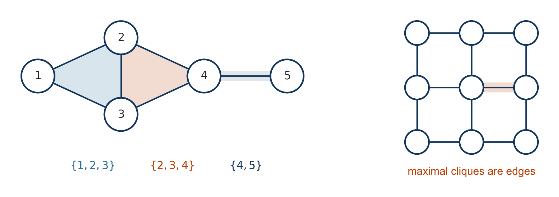
- An undirected graph \(G = (V, E)\): nodes \(V = \{1, \ldots, n\}\), one per variable, and a set \(E\) of unordered pairs. The neighbours of \(i\) are \(\mathcal{N}(i) = \{j : \{i, j\} \in E\}\). On the left, \(\mathcal{N}(4) = \{2, 3, 5\}\).
- A clique is a set of nodes every two of which are joined by an edge. Single nodes and edges count. On the left, \(\{1, 2, 3\}\) is a clique and \(\{1, 2, 3, 4\}\) is not, since \(1\) and \(4\) are not adjacent.
- A clique is maximal if no node can be added to it. On the left the maximal cliques are \(\{1, 2, 3\}\), \(\{2, 3, 4\}\) and \(\{4, 5\}\). Every clique sits inside a maximal one.
- On a grid there are no triangles, so the maximal cliques are exactly the edges. That is why the Ising model will have only pairwise potentials.
Potentials and the normalizer
An undirected graphical model, or Markov random field, on variables \(\mathbf{x} = (x_1, \ldots, x_n)\) is
\[
p(\mathbf{x}) = \frac{1}{Z} \prod_{C} \psi_C(\mathbf{x}_C),
\qquad
Z = \sum_{\mathbf{x}} \prod_{C} \psi_C(\mathbf{x}_C),
\]
with one nonnegative potential \(\psi_C\) per clique \(C\) of the graph. For continuous variables replace the sum by an integral over \(\mathbf{x}\). Everything in this lecture is discrete, so sums throughout.
- A potential is a compatibility score, not a probability. It need not sum to one over anything.
- It is enough to use the maximal cliques: a potential on a smaller clique can be multiplied into a maximal clique that contains it. On the graph of the previous slide, \(\psi_1(x_1)\,\psi_{12}(x_1, x_2)\,\psi_{123}(x_1, x_2, x_3)\) is a function of \((x_1, x_2, x_3)\) alone, so it is one potential on \(\{1, 2, 3\}\). On a grid that leaves one potential per edge.
- A directed model is normalized locally: each factor is a conditional distribution, so the product sums to one automatically. An undirected model is normalized globally, by \(Z\).
- \(Z\) is a sum over every joint configuration.
Reading independence off the graph
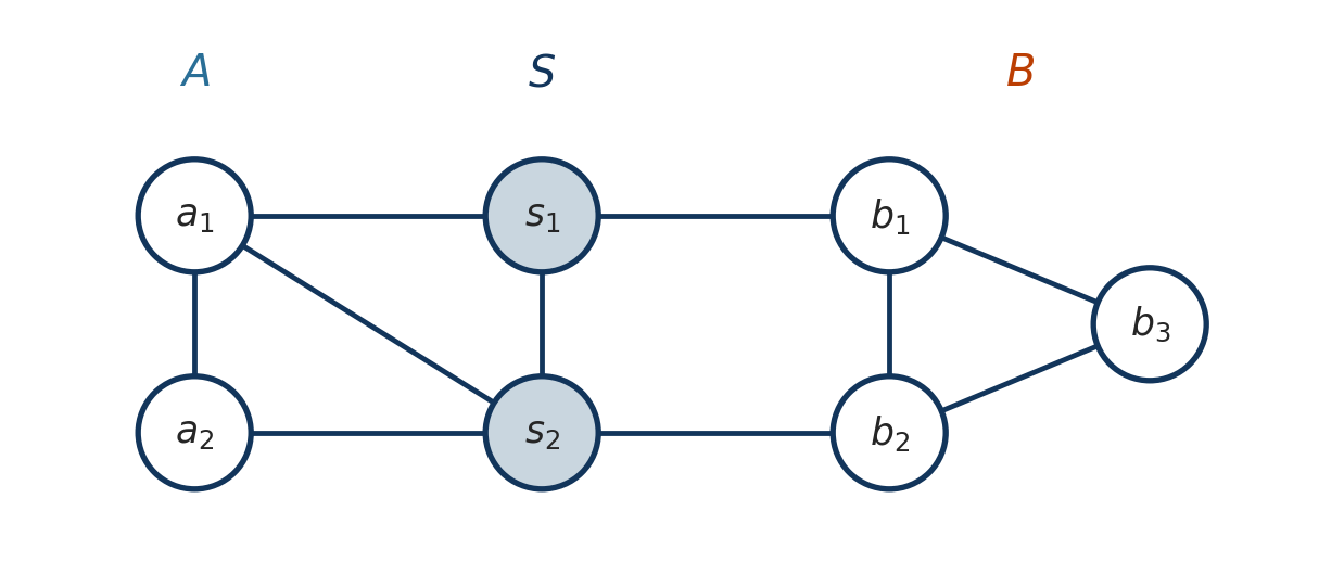
Separation. \(\mathbf{x}_A \perp \mathbf{x}_B \mid \mathbf{x}_S\) whenever every path from \(A\) to \(B\) passes through \(S\).
- Simpler than Bayes ball: no arrows, so no v-structures and no explaining away. Observing a node only ever blocks paths.
- In particular, a variable is independent of everything else given its neighbours, its Markov blanket.
What the theorem buys you
For a positive distribution, the graph’s independences and the clique factorization are the same thing. So there are two ways to specify a model, and they agree.
- Draw the graph, write the potentials. Any product of nonnegative clique potentials respects every independence the graph shows. Nothing to check. This is how the Ising model is written.
- Start from the local conditionals. Instead of a joint, specify for each \(i\) how \(x_i\) depends on its neighbours, \(p(x_i \mid \mathbf{x}_{\mathcal{N}(i)})\). The theorem says any positive joint with these conditionals is a product of clique potentials on the graph. So the two descriptions never disagree, and we can pass between them freely.
- What it does not give is \(Z\). The factorization exists; computing its normalizer is a separate problem.
The Ising model
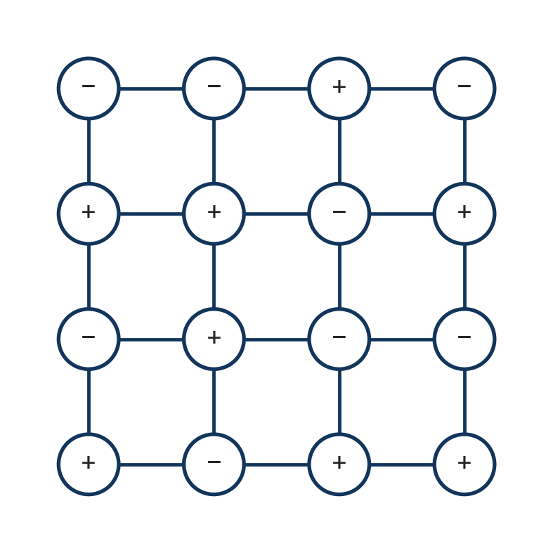
Spins \(x_i \in \{-1, +1\}\) on an \(n \times n\) grid, edges between horizontal and vertical neighbours, free boundary:
\[
p(\mathbf{x}) = \frac{1}{Z(\beta)} \exp\Big( \beta \sum_{i \sim j} x_i x_j + h \sum_i x_i \Big).
\]
- One potential per edge, \(\psi_{ij}(x_i, x_j) = e^{\beta x_i x_j}\): worth \(e^{\beta}\) when the neighbours agree and \(e^{-\beta}\) when they disagree. The optional field \(h\) adds a unary potential \(e^{h x_i}\) that favours \(+1\); today \(h = 0\) unless stated.
- In physics the exponent is minus an energy, \(E(\mathbf{x}) = -J \sum_{i \sim j} x_i x_j - H \sum_i x_i\), and \(p(\mathbf{x}) \propto e^{-E(\mathbf{x}) / k_B T}\) is the Boltzmann distribution at temperature \(T\). Low energy means high probability, and lowering \(T\) sharpens the distribution. Any positive \(p\) can be written this way with \(E = -\log p\), which is why \(-\log \psi_C\) is often called the energy of a clique.
What \(\beta\) does
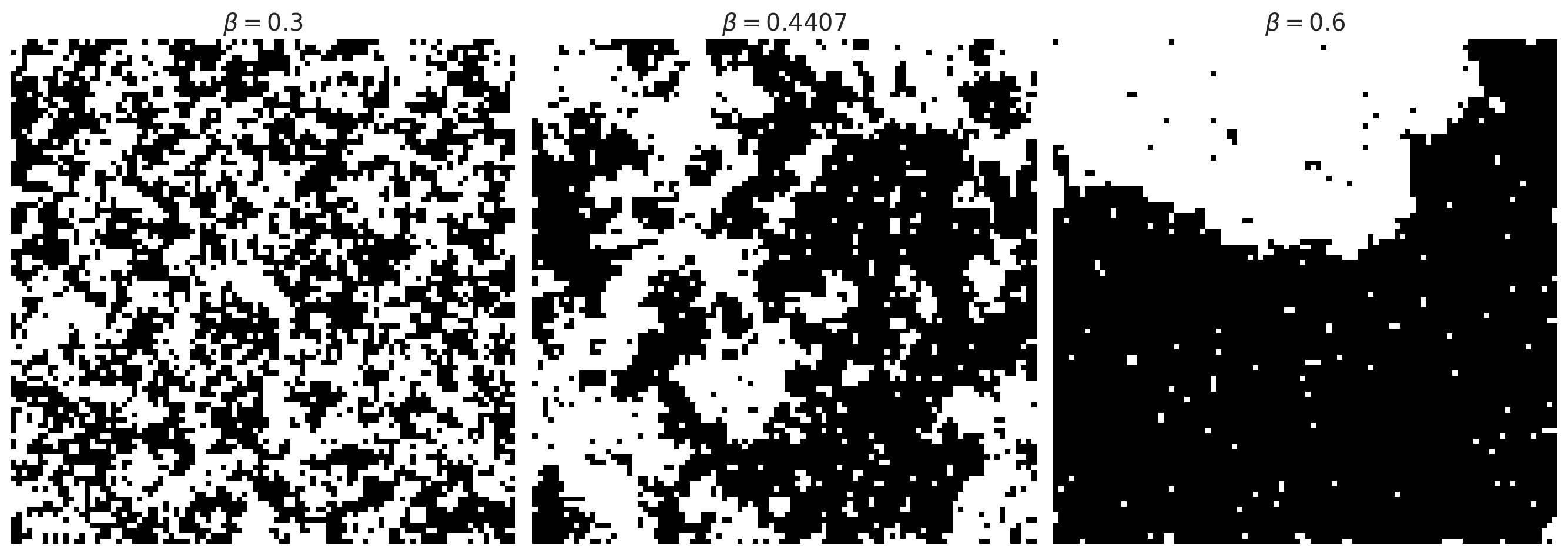
- Three configurations of a \(96 \times 96\) Ising model at \(h = 0\), each produced by the method we arrive at by the end of this lecture, run for 400 sweeps from a random start. Same potentials, three couplings.
- \(\beta \ge 0\) is the coupling, an inverse temperature. At \(\beta = 0\) the spins are independent coin flips; as \(\beta\) grows, agreement is rewarded more.
- On an infinite grid there is a sharp transition at \(\beta_c = \tfrac12 \log(1 + \sqrt 2) \approx 0.4407\) (Onsager, 1944): below it, local disorder; above it, large aligned domains.
Brute force on small grids
Enumerate every configuration, \(2^9 = 512\) for \(3 \times 3\) and \(2^{16} = 65{,}536\) for \(4 \times 4\), to get \(Z\) and three expectations: two neighbouring spins, two opposite corners, and \(m^2\) for the mean spin \(m\).
| 3 x 3 |
0.2 |
653.959 |
0.2053 |
0.0093 |
0.2006 |
| 3 x 3 |
0.44 |
1804.52 |
0.4900 |
0.1757 |
0.4364 |
| 3 x 3 |
0.7 |
14508.2 |
0.7857 |
0.5948 |
0.7638 |
| 4 x 4 |
0.2 |
107106 |
0.2054 |
0.0013 |
0.1260 |
| 4 x 4 |
0.44 |
862467 |
0.4955 |
0.1093 |
0.3702 |
| 4 x 4 |
0.7 |
7.31168e+07 |
0.8066 |
0.5922 |
0.7910 |
- Neighbours are about equally correlated on both grids. The corner-to-corner correlation, and \(\mathbb{E}[m^2]\), depend on the size of the grid, and at \(\beta = 0.7\) the whole grid tends to align.
What it costs
| 3 x 3 |
512 |
0.00014 seconds |
| 4 x 4 |
6.55e+04 |
0.0179 seconds |
| 5 x 5 |
3.36e+07 |
9.16 seconds |
| 6 x 6 |
6.87e+10 |
5.21 hours |
| 10 x 10 |
1.27e+30 |
1.1e+16 years |
- The \(4 \times 4\) timing, extrapolated at a fixed cost per configuration. A \(5 \times 5\) grid would also need about 7 GB just to hold the configurations.
- The age of the universe is about \(1.4 \times 10^{10}\) years. A \(10 \times 10\) grid is tiny; a small image is \(256 \times 256\).
- In the HMM lecture, \(K^n\) terms collapsed to \(O(nK^2)\) because fixing one variable split the sum. No single spin splits a grid; the smallest set that does is a whole row of \(n\) spins, with \(2^n\) ways to fix it.
How would you sample from it?
What we have: \(p(\mathbf{x})\) up to \(Z\). We can evaluate \(\exp(\beta \sum_{i \sim j} x_i x_j)\) for any \(\mathbf{x}\), but \(Z\) itself is out of reach.
What we want: draws \(\mathbf{x}^{(1)}, \ldots, \mathbf{x}^{(S)}\) from \(p\), so that averages estimate expectations.
Hint: one spin given all the others
Fix a site \(i\). Starting from \(p(\mathbf{x}) = \tfrac{1}{Z} \exp(\beta \sum_{j \sim k} x_j x_k)\), write down \(p(x_i \mid \mathbf{x}_{-i})\). Which factors cancel between numerator and denominator? What is left, and what does it depend on?
- \(p(x_i \mid \mathbf{x}_{-i}) = p(\mathbf{x}) / \sum_{x_i} p(\mathbf{x})\). The denominator sums over the two values of one spin.
- \(Z\) cancels. So does every edge factor \(e^{\beta x_j x_k}\) that does not involve \(x_i\). What is left is \(e^{\beta x_i s_i}\), where \(s_i = \sum_{j \in \mathcal{N}(i)} x_j\) is the sum of the neighbouring spins, so \[
p(x_i = +1 \mid \mathbf{x}_{-i}) = \frac{e^{\beta s_i}}{e^{\beta s_i} + e^{-\beta s_i}} = \sigma(2 \beta s_i), \qquad \sigma(u) = \frac{1}{1 + e^{-u}}.
\]
- The same formula holds at every site; an edge or corner site has fewer neighbours.
- This is the separation statement read off the graph earlier, \(x_i \perp \mathbf{x}_{\text{rest}} \mid \mathbf{x}_{\mathcal{N}(i)}\), now as a formula you can draw from. Read the other way, these conditionals at every site are the second description on the Hammersley–Clifford slide, and the theorem says the joint they describe is the product of edge potentials we started from.
What can you do with one conditional?
You cannot draw \(x_i\) from \(p(x_i)\), but you can draw it from \(p(x_i \mid \mathbf{x}_{-i})\). Start from any configuration, pick a site, redraw that one spin from its conditional, and repeat. Does this produce draws from \(p\)? Why might it, and what could go wrong?
- Two questions to settle. If \(\mathbf{x}\) is already a draw from \(p\) and you redraw one spin from its conditional, is the result still a draw from \(p\)?
- And if you start from an arbitrary configuration and redraw one site at a time, in some order, for a long time. Will the result be a draw from \(p\)?