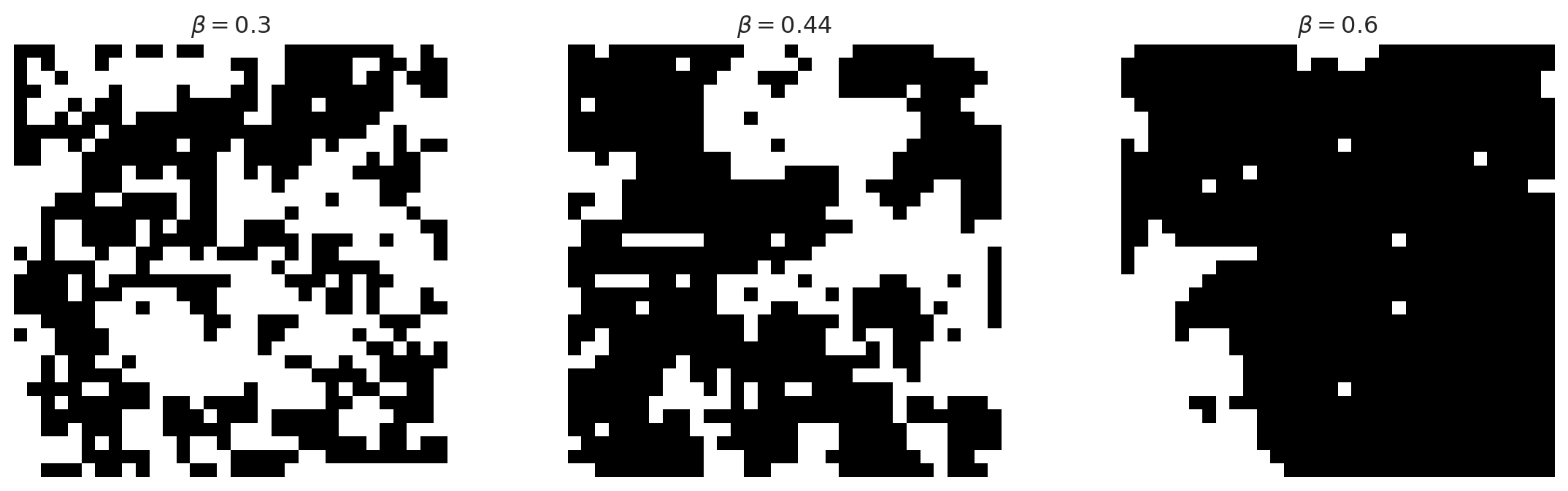
Today you will turn that equation into two samplers and determine whether their output is trustworthy.
Goals
Implement Gibbs sampling one site at a time.
Use conditional independence to update half the lattice simultaneously with block Gibbs.
Validate both samplers against exact answers on a \(3\times3\) lattice.
Diagnose dependent output using trace plots and multiple-chain split \(\hat R\).
Setup and conventions
import numpy as npimport pandas as pdimport matplotlib.pyplot as pltimport seaborn as snsimport timerng = np.random.default_rng(7)sns.set_style("whitegrid")INK, OBS, M1 ="#12355b", "#c9d6df", "#2a6f97"
A state is an n x n numpy array containing only -1 and +1.
We use free boundaries: a corner has two neighbours, a non-corner boundary site has three, and an interior site has four.
One sweep means that every site has been updated once.
Functions update x in place and return it, so call them with x.copy() when the original is needed.
Files and workflow
Put the implementation in a Python module named lab6.py. It should contain the functions developed in this lab, including the single-site and block Gibbs updates and split_rhat.
Create lab6.qmd for the experiments and write-up. Import your functions from lab6.py, and include the checks, figures, timing results, and written answers. Develop and test lab6.py first; render the complete document once the functions pass the checks.
You may test lab6.py interactively in either environment:
Run individual Python cells from your Quarto editor.
Use a Python console or a temporary Jupyter notebook to import the module and try small examples. The notebook is scratch work, not part of the submission.
If you test in JupyterLab, automatic reloading lets the notebook see edits to lab6.py without restarting its kernel:
%load_ext autoreload%autoreload 2
Single-site Gibbs
Task 1: sum the neighbours
Implement the neighbour sum \(s_i\) of the site stored at x[i, j], without wrapping across the boundary.
def local_neighbour_sum(x, i, j):"""Sum the up, down, left and right neighbours of x[i, j]."""# TODO: include only neighbours that are inside the arrayraiseNotImplementedError
Check an interior site, a corner, and a non-corner boundary site:
Given \(s_i\), draw a new value from the full conditional. This is a Gibbs draw, not a proposal followed by an acceptance decision.
def gibbs_site(x, i, j, beta, rng):"""Draw x[i, j] from its full conditional and update x in place.""" s = local_neighbour_sum(x, i, j)# TODO: compute p(x[i, j] = +1 | neighbours)# TODO: use rng.random() to draw +1 or -1, and assign the result to x[i, j]raiseNotImplementedError
Note
The old value of x[i, j] does not enter the full conditional. Gibbs draws a new value from the full conditional, so the spin may either stay the same or change.
Does the conditional behave sensibly?
For an interior site, \(s_i\in\{-4,-2,0,2,4\}\). Compute the probability of a positive spin at each possible value.
for beta in [0.3, 0.44, 0.6]: probs = [1/ (1+ np.exp(-2* beta * s)) for s in [-4, -2, 0, 2, 4]]print(f"beta={beta:.2f}:", np.round(probs, 3))
Larger \(\beta\) makes the neighbours more influential.
Task 3: one single-site sweep
Visit every site once. We use a fresh random order so that no site is always updated first or last.
def single_site_sweep(x, beta, rng):"""Update every site once, in a random order.""" nrow, ncol = x.shape# TODO: loop over rng.permutation(nrow * ncol)# TODO: convert a flat index k to (i, j) with divmod(k, ncol)# TODO: call gibbs_siteraiseNotImplementedError
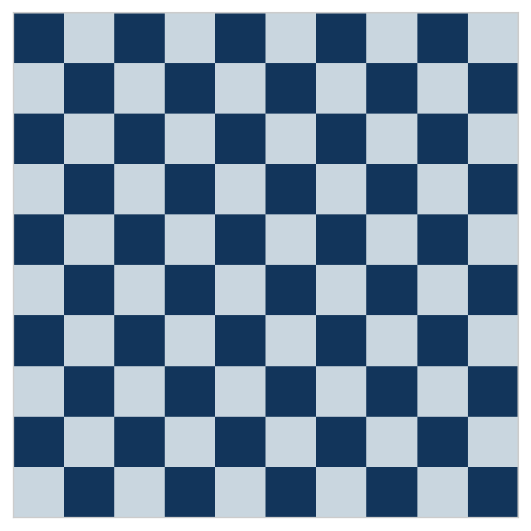
We can therefore draw every dark spin simultaneously, then recompute the neighbour sums and draw every light spin simultaneously.
All neighbour sums at once
Use zero padding and array slices to produce an array s with the same shape as x.
def neighbour_sum(x):"""Array whose [i, j] entry is the sum of the neighbours of x[i, j].""" p = np.pad(x, 1)return (p[:-2, 1:-1] +# above p[2:, 1:-1] +# below p[1:-1, :-2] +# left p[1:-1, 2:]) # right
dark_mask is a Boolean array: it is True at dark sites and False at light sites. np.logical_not(dark_mask) reverses those values to create light_mask.
def block_gibbs_sweep(x, beta, rng, dark_mask):"""Update the dark block given light, then light given the new dark block.""" light_mask = np.logical_not(dark_mask)for mask in (dark_mask, light_mask):# TODO: recompute all neighbour sums# TODO: compute every p(x_i = +1 | neighbours)# TODO: draw an array of +1/-1 values# TODO: overwrite x only where mask is TrueraiseNotImplementedErrorreturn x
Important
Recompute the neighbour sums between the two half-sweeps. The light update must condition on the new dark spins, not the old ones.
Single-site and block Gibbs target the same distribution
On a \(3\times3\) lattice there are only \(2^9=512\) states, so expectations under \(p\) can be computed exactly by enumeration. We compare three of them at \(\beta=0.44\): the adjacent pair x[0, 0] * x[0, 1], the opposite corners x[0, 0] * x[2, 2], and the squared magnetization x.mean() ** 2.
single-site: 27.07 ms per sweep
block:       0.30 ms per sweep
speedup:     90.0x
Both methods update every spin from the same full conditional. The speedup is computational: numpy performs a few whole-array operations instead of thousands of Python-level updates.
Dependent draws
A helper for running one chain
Add this provided helper to lab6.py. It runs burn-in and then records one magnetization value per sweep.
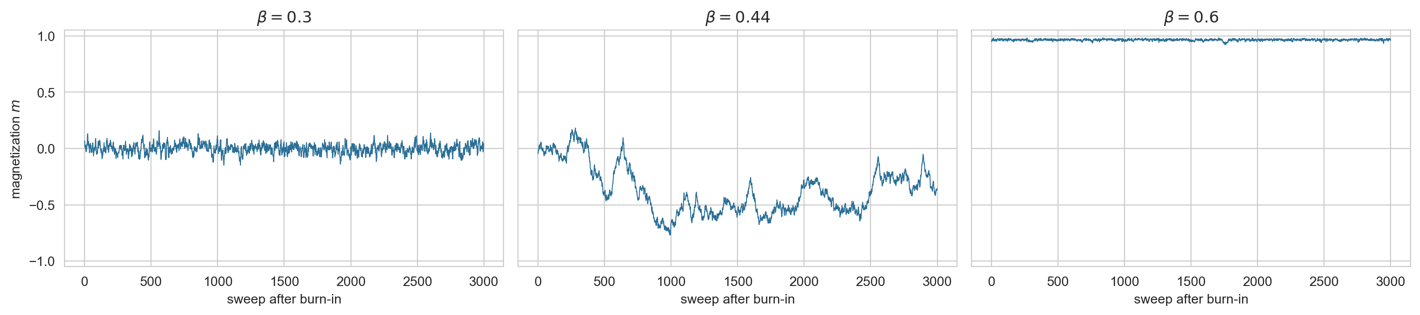
Describe what changes as \(\beta\) approaches and passes the critical value \(\beta_c\approx0.4407\). For each trace identify its center, range, trends, and persistence. Burn-in is a guess, not a guarantee: check the start of each trace for a leftover transient, and if one remains, say that the burn-in was too short.
Multiple chains and \(\hat R\)
Why one chain is not enough
A trace can look stable because it is trapped in one region. Run several chains from deliberately different starting points.
If the chains explore the same target, their between-chain variation should eventually resemble their within-chain variation.
If chains remain separated, the between-chain variation is too large.
Agreement does not prove convergence, but disagreement is direct evidence of failure.
Split \(\hat R\)
Suppose each of the \(M\) original chains contains \(L\) draws. Split each chain in half, giving \(2M\) sequences of length \(T=\lfloor L/2\rfloor\). For split chain \(j\), let \(\bar f_j\) be its sample mean and \(s_j^2\) its sample variance. Let \(\operatorname{Var}(\bar f_1,\ldots,\bar f_{2M})\) denote the sample variance across the \(2M\) chain means. Then
Values appreciably above one indicate that the chains do not yet agree.
Task 6: implement split \(\hat R\)
def split_rhat(chains):"""chains has shape (number of chains, draws per chain).""" chains = np.asarray(chains, dtype=float) n_chains, n_draws = chains.shape n_half = n_draws //2# TODO: concatenate the first and last n_half draws as 2*n_chains split chains# TODO: compute W, B, V_hat and return sqrt(V_hat / W)raiseNotImplementedError
This is the classical split-\(\hat R\) calculation. Modern software additionally rank-normalizes and folds the draws, but the between-versus-within-chain logic is the same.
Chains started in opposite phases
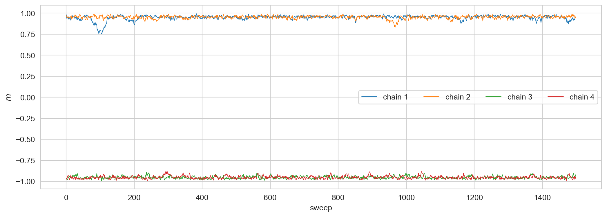
Run two chains from all \(+1\) and two from all \(-1\) at \(\beta=0.6\). A \(32\times32\) lattice keeps the run short; the behaviour is the same on the \(64\times64\) lattice.
None of them proves that all important regions were visited.
For the \(\beta=0.6\) Ising model, local updates have trouble reversing the sign of an entire ordered lattice. More iterations do not automatically repair a sampler whose relevant transition is extraordinarily rare.
Checklist before you submit
What to submit
Submit:
lab6.py, containing the implementations and provided helper functions used by Tasks 1–6.
lab6.qmd, containing all checks, figures, timing results, and the written answers below.
Written answers, one short paragraph each:
Trace plots (Task 5): for each \(\beta\), the center, range, trends, and persistence of the trace, and whether a transient remains after burn-in.
Computing time: whether block Gibbs mixes faster per sweep, and what the speedup does and does not change.
Chains in opposite phases: why \(\hat R\) is poor for \(m\) but close to one for \(|m|\), and what feature of the target the absolute value hides.
The report must run using functions imported from lab6.py; do not duplicate their implementations in the report. Discuss freely; write your own code.
Backup slides
Why \(\hat R\) approaches one
Suppose every split chain has reached the same stationary distribution, with mean \(\mu\) and variance \(\sigma^2\).
The average within-chain variance estimates the target variance: \[W\approx\sigma^2.\]
As the chains run longer, their means concentrate near the same \(\mu\), so \[\frac{B}{T}=\operatorname{Var}(\bar f_1,\ldots,\bar f_{2M})\longrightarrow0.\]
For independent stationary draws, \(\operatorname{Var}(\bar f_j)=\sigma^2/T\), so \(B\approx\sigma^2\) and \(\hat R\approx1\) at any \(T\). For a chain with integrated autocorrelation time \(\tau\), \(\operatorname{Var}(\bar f_j)\approx\tau\sigma^2/T\), so \(B\approx\tau\sigma^2\) and
\[
\hat R\approx\sqrt{1+\frac{\tau-1}{T}}.
\]
This is why \(\hat R\) stays slightly above one for a finite run even when every chain is stationary, and why it approaches one as \(T\) grows.
Why \(\hat R\) can be large
Suppose some chains are trapped near \(+1\) and others near \(-1\).
Each chain may fluctuate very little, making the within-chain variance \(W\) small.
The chain means are far apart, making the between-chain estimate \(B\) large.
Therefore \(\widehat V>W\) and \(\hat R>1\).
Splitting also compares the first and second halves of each chain, so a chain that is drifting can disagree with itself.
Important
\(\hat R\approx1\) means that the chains agree; it does not prove convergence. All chains could be trapped in the same mode.
Autocorrelation
For a scalar trace \(f_t=f(\mathbf{x}^{(t)})\), the lag-\(k\) autocorrelation measures how much knowing \(f_t\) predicts \(f_{t+k}\):
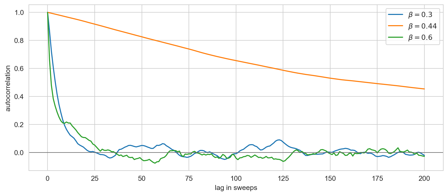
The two calculations agree; the FFT is only a computational shortcut. Slowly decaying \(\rho_k\) means that many recorded states contain nearly the same information.
Autocorrelation of magnetization
fig, ax = plt.subplots(figsize=(9, 4))for beta in BETAS: ax.plot(autocorrelation(traces[beta])[:201], label=f"$\\beta={beta}$")ax.axhline(0, color="0.4", lw=0.8)ax.set_xlabel("lag in sweeps"); ax.set_ylabel("autocorrelation")ax.legend(); plt.tight_layout(); plt.show()
Effective sample size
The integrated autocorrelation time and effective sample size for the function \(f\) are
Starting with \(k=0\), keep the longest initial sequence for which every \(\widehat G_k>0\); stop before the first nonpositive pair. If \(m\) is the final retained index, estimate
Geyer’s positivity result is for reversible chains. A fixed dark-then-light Gibbs sweep leaves \(p\) invariant but need not itself be reversible; the estimator is included here as a common reference method, not as a required diagnostic for this lab.