Probabilistic Machine Learning

Markov chain Monte Carlo

Seong-Hwan Jun

Department of Biostatistics and Computational Biology, University of Rochester Medical Center

Where we left off

The Ising model on an \(n \times n\) grid with spins \(x_i \in \{-1, +1\}\):

\[ p(\mathbf{x}) = \frac{1}{Z(\beta)} \exp\Big(\beta \sum_{i \sim j} x_i x_j\Big), \qquad Z(\beta) = \sum_{\mathbf{x}} \exp\Big(\beta \sum_{i \sim j} x_i x_j\Big). \]

\(Z\) is a sum over \(2^{n^2}\) configurations. Enumerating \(3 \times 3\) and \(4 \times 4\) was feasible; \(10 \times 10\) is \(2^{100}\).
One spin given all the others: in \(p(x_i \mid \mathbf{x}_{-i}) = p(\mathbf{x}) / \sum_{x_i} p(\mathbf{x})\) every factor without \(x_i\) cancels, and so does \(Z\). What is left involves only the four neighbours, through their sum \(s_i = \sum_{j \sim i} x_j\): \[ p(x_i = +1 \mid \mathbf{x}_{-i}) = \sigma(2 \beta s_i), \qquad \sigma(u) = \frac{1}{1 + e^{-u}}. \]
No \(Z\) in it. Today we turn that one fact into samples from \(p(\mathbf{x})\), and the samples into expectations.

Goals

Define a Markov chain’s stationary distribution, and show that detailed balance is enough to have one.
Derive Metropolis-Hastings, prove it leaves the target invariant, and see why it never needs \(Z\).
Show that Gibbs sampling is Metropolis-Hastings that always accepts. We will implement a vectorized block Gibbs sampler for the Ising model in the lab.

Markov chains

The plan

Many questions about a distribution can be written as expectations:

\[ \Pr_p(\mathbf{x} \in A) = \mathbb{E}_p[\mathbf{1}\{\mathbf{x} \in A\}], \qquad \operatorname{Cov}_p(x_i, x_j) = \mathbb{E}_p[x_i x_j] - \mathbb{E}[x_i] \mathbb{E}[x_j]. \]

Our computational goal is to estimate \(\mathbb{E}_p[f(\mathbf{x})]\) for functions \(f\) of interest, even when we cannot draw independent samples from \(p\).

Build a sequence \(\mathbf{x}^{(0)}, \mathbf{x}^{(1)}, \ldots\) in which each state is a random perturbation of the last, designed so that in the long run the states are distributed according to \(p\).
Average \(f\) along the sequence.
The draws are dependent, so two questions: why does this converge to the right thing, and how many dependent draws are worth one independent one?

A Markov chain

For every current state \(\mathbf{x}\), a transition kernel \(T(\cdot \mid \mathbf{x})\) is a probability distribution over the next state \(\mathbf{x}'\):

\[ T(\mathbf{x}' \mid \mathbf{x}) \geq 0, \qquad \sum_{\mathbf{x}'} T(\mathbf{x}' \mid \mathbf{x}) = 1. \]

Run the chain by repeatedly drawing from this distribution:

\[ \mathbf{x}^{(t+1)} \sim T(\cdot \mid \mathbf{x}^{(t)}). \]

On a finite space, \(T\) is a matrix with rows summing to one: \(T_{x x'} = T(x' \mid x)\). If \(q_t\) is the distribution of \(\mathbf{x}^{(t)}\), written as a row vector, then \(q_{t+1} = q_t T\).
On a continuous space it is a conditional density, and the matrix product becomes \(q_{t+1}(\mathbf{x}') = \int q_t(\mathbf{x}) \, T(\mathbf{x}' \mid \mathbf{x}) \, d\mathbf{x}\).
We get to design \(T\).

Stationary distribution

A distribution \(\pi\) is stationary (or invariant) for \(T\) if one step leaves it unchanged:

\[ \pi(\mathbf{x}') = \sum_{\mathbf{x}} \pi(\mathbf{x}) \, T(\mathbf{x}' \mid \mathbf{x}) \quad \text{for every } \mathbf{x}', \qquad \text{i.e. } \pi T = \pi. \]

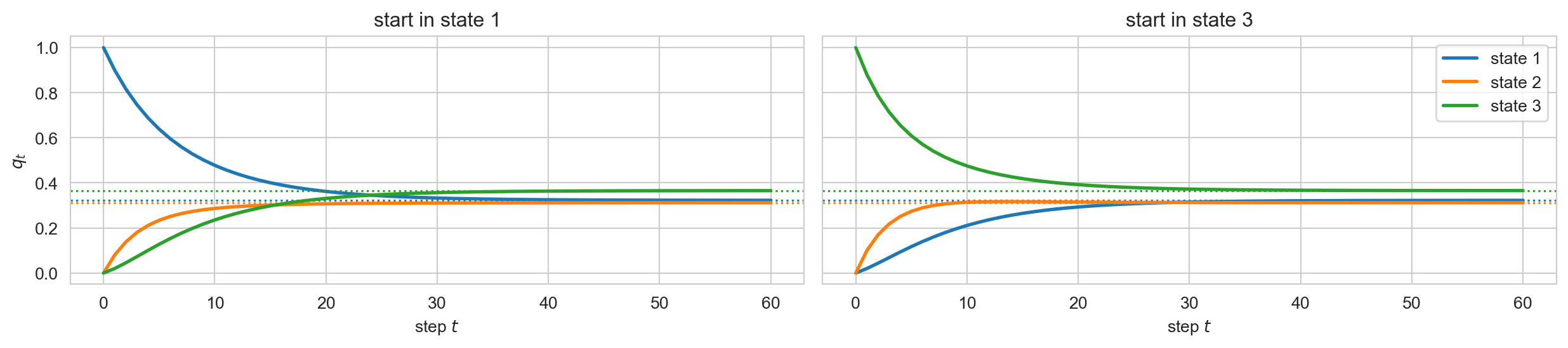
The regime chain from Assignment 2, started in two different states. The distribution of the state forgets where it began and settles at \(\pi\) (dotted). MCMC turns this around: choose \(T\) so that the \(\pi\) it settles at is the \(p\) we want.

Detailed balance

\(T\) satisfies detailed balance with respect to \(\pi\) if, for every pair of states,

\[ \pi(\mathbf{x}) \, T(\mathbf{x}' \mid \mathbf{x}) = \pi(\mathbf{x}') \, T(\mathbf{x} \mid \mathbf{x}'). \]

The flow from \(\mathbf{x}\) to \(\mathbf{x}'\) equals the flow back. It implies stationarity in one line: sum both sides over \(\mathbf{x}\),

\[ \sum_{\mathbf{x}} \pi(\mathbf{x}) \, T(\mathbf{x}' \mid \mathbf{x}) = \pi(\mathbf{x}') \sum_{\mathbf{x}} T(\mathbf{x} \mid \mathbf{x}') = \pi(\mathbf{x}'). \]

Detailed balance is a sufficient, but not necessary, condition for stationarity. It is a condition on pairs of states, which we can check one proposal at a time; stationarity is a condition on a sum over the whole space.
Two more conditions make the chain converge to \(\pi\) from any start: irreducible (every state can reach every other) and aperiodic (no deterministic cycling). Both are usually easy to arrange.

Metropolis-Hastings

The algorithm

Target \(p(\mathbf{x}) = \tilde p(\mathbf{x}) / Z\), known up to \(Z\). Proposal \(q(\mathbf{x}' \mid \mathbf{x})\), anything we can sample from. Initialize \(\mathbf{x}\).

Propose \(\mathbf{x}' \sim q(\cdot \mid \mathbf{x})\).
Compute \[ \alpha(\mathbf{x} \to \mathbf{x}') = \min\left(1, \; \frac{\tilde p(\mathbf{x}') \, q(\mathbf{x} \mid \mathbf{x}')}{\tilde p(\mathbf{x}) \, q(\mathbf{x}' \mid \mathbf{x})}\right). \]
With probability \(\alpha\) move to \(\mathbf{x}'\); otherwise stay at \(\mathbf{x}\), and record \(\mathbf{x}\) again.

\(Z\) appears in numerator and denominator and cancels. This is the whole reason MCMC exists: it needs ratios of \(p\), never \(p\) itself.
Symmetric proposal, \(q(\mathbf{x}' \mid \mathbf{x}) = q(\mathbf{x} \mid \mathbf{x}')\): the ratio is \(\tilde p(\mathbf{x}') / \tilde p(\mathbf{x})\). Uphill moves are always accepted, downhill ones sometimes. This is the original Metropolis algorithm (1953), and it was invented for exactly this kind of lattice model.

Why it works

Claim. The Metropolis-Hastings kernel satisfies detailed balance with respect to \(p\), and therefore leaves \(p\) stationary.

The kernel. For \(\mathbf{x}' \neq \mathbf{x}\) the chain lands on \(\mathbf{x}'\) only by proposing it and accepting, so \[ T(\mathbf{x}' \mid \mathbf{x}) = q(\mathbf{x}' \mid \mathbf{x})\, \alpha(\mathbf{x} \to \mathbf{x}'), \qquad \alpha(\mathbf{x} \to \mathbf{x}') = \min\left(1,\; \frac{p(\mathbf{x}')\, q(\mathbf{x} \mid \mathbf{x}')}{p(\mathbf{x})\, q(\mathbf{x}' \mid \mathbf{x})}\right), \] and \(T(\mathbf{x} \mid \mathbf{x}) = 1 - \sum_{\mathbf{x}' \neq \mathbf{x}} q(\mathbf{x}' \mid \mathbf{x})\, \alpha(\mathbf{x} \to \mathbf{x}')\) collects every rejection.

Detailed balance: forward and reverse moves

Fix \(\mathbf{x}' \neq \mathbf{x}\) and suppose both proposal flows are positive. Define the Hastings ratio for the move \(\mathbf{x} \to \mathbf{x}'\): \[ r = \frac{p(\mathbf{x}')q(\mathbf{x} \mid \mathbf{x}')} {p(\mathbf{x})q(\mathbf{x}' \mid \mathbf{x})}. \]

For the reverse move \(\mathbf{x}' \to \mathbf{x}\), the ratio is \(1/r\). Therefore \[ \alpha(\mathbf{x} \to \mathbf{x}') = \min(1,r), \qquad \alpha(\mathbf{x}' \to \mathbf{x}) = \min(1,1/r). \]

We must show that the probability flow is the same in both directions: \[ p(\mathbf{x})T(\mathbf{x}' \mid \mathbf{x}) =p(\mathbf{x}')T(\mathbf{x} \mid \mathbf{x}'). \]

Detailed balance: case 1

Suppose \(r \leq 1\). The forward move is accepted with probability \(r\), while the reverse move is accepted with probability \(1\) because \(1/r \geq 1\). Thus \[ \begin{aligned} p(\mathbf{x})T(\mathbf{x}' \mid \mathbf{x}) &=p(\mathbf{x})q(\mathbf{x}' \mid \mathbf{x}) \alpha(\mathbf{x} \to \mathbf{x}') \\ &=p(\mathbf{x})q(\mathbf{x}' \mid \mathbf{x})r \\ &=p(\mathbf{x}')q(\mathbf{x} \mid \mathbf{x}') \\ &=p(\mathbf{x}')q(\mathbf{x} \mid \mathbf{x}') \alpha(\mathbf{x}' \to \mathbf{x}) \\ &=p(\mathbf{x}')T(\mathbf{x} \mid \mathbf{x}'). \end{aligned} \]

The second last line \(\alpha(\mathbf{x}' \to \mathbf{x}) = \min(1, 1/r) = 1\) since \(1/r \geq 1\).

Detailed balance: case 2

Suppose \(r > 1\). The forward move is accepted with probability \(1\), while the reverse move is accepted with probability \(1/r\) because \(1/r < 1\). Thus \[ \begin{aligned} p(\mathbf{x})T(\mathbf{x}' \mid \mathbf{x}) &=p(\mathbf{x})q(\mathbf{x}' \mid \mathbf{x}) \alpha(\mathbf{x} \to \mathbf{x}') \\ &=p(\mathbf{x})q(\mathbf{x}' \mid \mathbf{x}) \\ &=p(\mathbf{x}')q(\mathbf{x} \mid \mathbf{x}')\frac{1}{r} \\ &=p(\mathbf{x}')q(\mathbf{x} \mid \mathbf{x}') \alpha(\mathbf{x}' \to \mathbf{x}) \\ &=p(\mathbf{x}')T(\mathbf{x} \mid \mathbf{x}'). \end{aligned} \]

For \(\mathbf{x}'=\mathbf{x}\), detailed balance is the identity \(p(\mathbf{x})T(\mathbf{x}\mid\mathbf{x})=p(\mathbf{x})T(\mathbf{x}\mid\mathbf{x})\).
Thus we have designed the MH transition kernel \(T\) to satisfy detailed balance with respect to \(p\). Because detailed balance implies stationarity, \(p\) is stationary for \(T\). \(\square\)

What the proof tells us

The ratio \(r\) contains \(p\) only as \(p(\mathbf{x}') / p(\mathbf{x})\), so \(Z\) cancels: the proof needs \(\tilde p\) only.
Nothing was assumed about \(q\) beyond being able to evaluate it. The proposal controls speed; the acceptance step guarantees correctness.
Rejections are part of the kernel. Dropping the repeated state when a proposal is rejected changes the stationary distribution.

Single spin flips

Let \(N=n^2\) be the number of sites. Choose \(i\) uniformly from the \(N\) sites and propose

\[ x_i'=-x_i, \qquad \mathbf{x}'_{-i}=\mathbf{x}_{-i}. \]

Therefore

\[ q(\mathbf{x}'\mid\mathbf{x})= \begin{cases} 1/N, & \mathbf{x}' \text{ differs from } \mathbf{x} \text{ at exactly one site},\\ 0, & \text{otherwise}. \end{cases} \]

The reverse move flips the same site, so \(q(\mathbf{x}'\mid\mathbf{x})=q(\mathbf{x}\mid\mathbf{x}')\). Only the four terms touching \(x_i\) change:

\[ \log \tilde p(\mathbf{x}') - \log \tilde p(\mathbf{x}) = \beta \sum_{j \sim i} (-x_i) x_j - \beta \sum_{j \sim i} x_i x_j = -2 \beta \, x_i \, s_i. \]

One proposal costs \(O(1)\) however large the grid: the structure of the model makes the ratio local.

quantity	\(\beta = 0.2\)	\(\beta = 0.44\)	\(\beta = 0.7\)
neighbours \(\mathbb{E}[x_{(0,0)} x_{(0,1)}]\)	0.2053	0.4900	0.7857
corners \(\mathbb{E}[x_{(0,0)} x_{(2,2)}]\)	0.0093	0.1757	0.5948
\(\mathbb{E}[m^2]\), \(m = \frac{1}{9}\sum_i x_i\)	0.2006	0.4364	0.7638

Metropolis on the \(3 \times 3\) grid

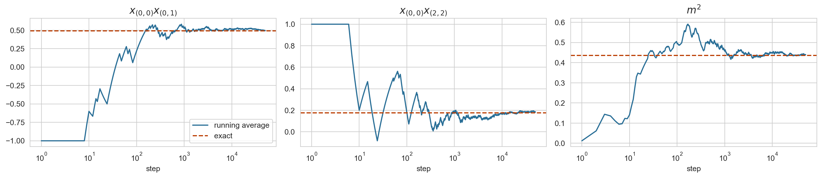
after 50,000 steps: neighbours 0.494 (exact 0.490)   corners 0.185 (exact 0.176)   m^2 0.440 (exact 0.436)

The running averages wander for the first few thousand steps and settle on the exact values. Nothing in the sampler knew \(Z\).
Suppose the state were recorded only when a flip is accepted. Which of the three quantities would be wrong, and in which direction?
The \(3 \times 3\) check is the last time we will have the truth. On a \(64 \times 64\) grid, the code has to be right before it runs.

Gibbs sampling

Gibbs is Metropolis-Hastings that always accepts

Propose a new value for one coordinate from its full conditional, keeping the rest:

\[ q(\mathbf{x}' \mid \mathbf{x}) = p(x'_i \mid \mathbf{x}_{-i}), \qquad \mathbf{x}'_{-i} = \mathbf{x}_{-i}. \]

Write \(p(\mathbf{x}) = p(x_i \mid \mathbf{x}_{-i}) \, p(\mathbf{x}_{-i})\), and likewise for \(\mathbf{x}'\), which has the same \(\mathbf{x}_{-i}\). The MH ratio is

\[ \frac{p(\mathbf{x}') \, q(\mathbf{x} \mid \mathbf{x}')}{p(\mathbf{x}) \, q(\mathbf{x}' \mid \mathbf{x})} = \frac{p(x'_i \mid \mathbf{x}_{-i}) \, p(\mathbf{x}_{-i}) \; p(x_i \mid \mathbf{x}_{-i})}{p(x_i \mid \mathbf{x}_{-i}) \, p(\mathbf{x}_{-i}) \; p(x'_i \mid \mathbf{x}_{-i})} = 1. \]

Every proposal is accepted, so there is no tuning: the proposal is the model’s own conditional.
The price: we must be able to sample the full conditional. In a model with local structure it involves only the variable’s neighbours. For the Ising model, \(p(x_i = +1 \mid \mathbf{x}_{-i}) = \sigma(2 \beta s_i)\).
Updating every coordinate once in a fixed order is a valid Gibbs sweep: each coordinate update leaves \(p\) invariant, so their composition does too. The full sweep need not be reversible, but reversibility is not required for stationarity.

Block Gibbs

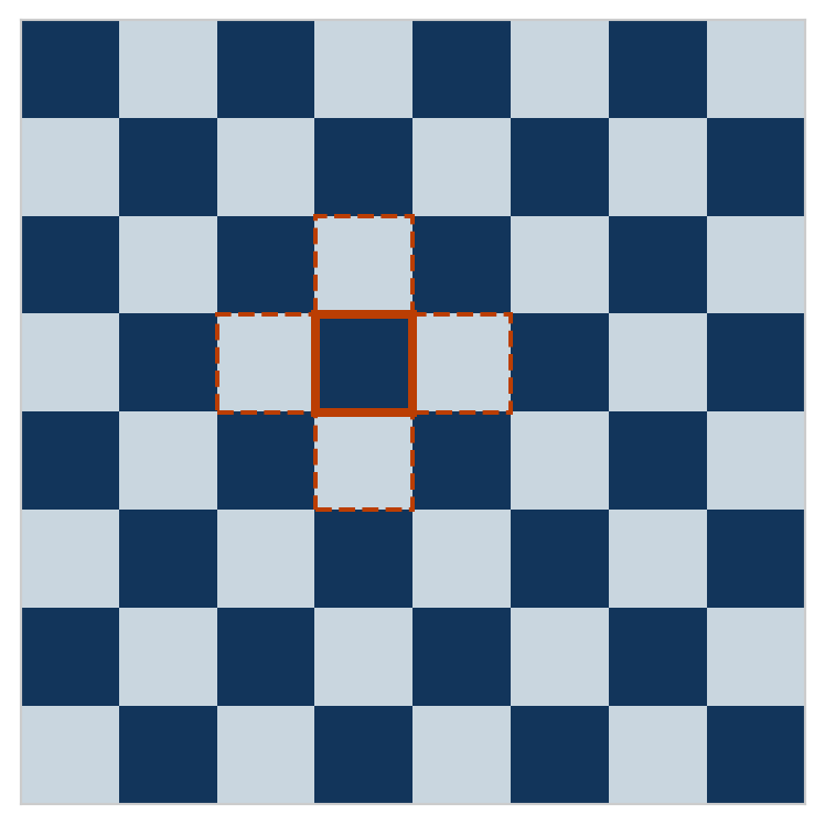
Colour the grid like a checkerboard. Every neighbour of a dark site is light, and vice versa: the grid graph is bipartite.
Given all the light spins, the dark spins are conditionally independent. No factor touches two dark sites, so \(p(\mathbf{x}_{\text{dark}} \mid \mathbf{x}_{\text{light}}) = \prod_{i \text{ dark}} p(x_i \mid \mathbf{x}_{\text{light}})\).
So half the grid can be drawn jointly and exactly in one vectorized step: a block Gibbs update. Two half sweeps make a full sweep.
The same separation statement read off the graph in the undirected models lecture. The gain is computational, not statistical: a sweep still draws every spin once from the same conditional, so the chain mixes no faster per sweep. But the draws of one colour are independent, so NumPy makes them in one array operation instead of a loop over sites, about 80 times faster per sweep on a \(64 \times 64\) grid.

The ergodic theorem and the MCMC CLT

For an irreducible, aperiodic chain with stationary distribution \(p\), started anywhere,

\[ \hat f_N = \frac{1}{N} \sum_{t=1}^{N} f(\mathbf{x}^{(t)}) \;\longrightarrow\; \mathbb{E}_p[f(\mathbf{x})] \quad \text{with probability one}. \]

Under mild extra conditions the error is again Gaussian, with a larger variance than for independent draws:

\[ \sqrt{N} \big( \hat f_N - \mathbb{E}_p[f] \big) \to \mathcal{N}\big(0, \; \sigma_f^2 \, \tau_f\big), \qquad \tau_f = 1 + 2 \sum_{k=1}^{\infty} \rho_k, \]

where \(\sigma_f^2 = \text{Var}_p[f]\) and \(\rho_k\) is the autocorrelation of \(f(\mathbf{x}^{(t)})\) at lag \(k\) once the chain is stationary.

\(\tau_f\), the integrated autocorrelation time, is the number of steps the chain needs to produce the equivalent of one independent draw.
The effective sample size is \(\text{ESS} = N / \tau_f\): the error of \(\hat f_N\) is that of an average of ESS independent draws.
It is a property of the chain and the function. The same run can have a large ESS for one \(f\) and a tiny one for another.

Exercise: Bayesian phylogenetics

The inference problem

We observe a DNA sequence alignment \(\mathbf{y}\) on a four-taxon tree. Fix the topology and every branch length except \(t_B\), the branch leading to taxon B.

From the belief-propagation lecture, pruning evaluates the likelihood

\[ L(t_B)=p(\mathbf{y}\mid t_B) \]

for any proposed value of \(t_B\). Our target is

\[ p(t_B\mid\mathbf{y}) \propto L(t_B)\,p(t_B), \qquad t_B>0. \]

What prior \(p(t_B)\) would make sense for a positive branch length? What would its scale or mean represent?

Design an MH update

Starting from a current branch length \(t>0\), design one Metropolis-Hastings update.

What proposal \(q(t'\mid t)\) would you use? How will it ensure that \(t'>0\)?
How will you evaluate the unnormalized posterior at \(t\) and \(t'\)?
What is the acceptance probability? Is your proposal symmetric on the scale of \(t\), or is a Hastings correction required?
What value do you record if the proposal is rejected?

Summary

What we have

idea	what it buys
detailed balance	a local check that the chain leaves \(p\) invariant
Metropolis-Hastings	a valid chain for any target known up to \(Z\), any proposal
Gibbs	MH with acceptance one, when full conditionals can be sampled
conditional independence	a full conditional that touches only neighbours, and blocks updated jointly
ESS	how many independent draws a dependent run is worth, for one function

Exact inference needed the sums to factor along a tree. MCMC needs only the ratio \(\tilde p(\mathbf{x}') / \tilde p(\mathbf{x})\), and the model’s structure makes that ratio local and cheap.
The cost moves from computation to convergence: an answer is only as good as the chain’s exploration, and the diagnostics can show failure but never prove success.

Reading

MCMC. Murphy, Probabilistic Machine Learning: Advanced Topics (2023), chapter 12, for the same material with diagnostics and ESS.
Optional. Geyer, “Introduction to Markov chain Monte Carlo”, chapter 1 of Brooks, Gelman, Jones and Meng (eds.), Handbook of Markov Chain Monte Carlo (2011): what the CLT does and does not promise, and why burn-in and thinning matter less than you might think.
History. Metropolis, Rosenbluth, Rosenbluth, Teller and Teller, “Equation of state calculations by fast computing machines”, Journal of Chemical Physics 21 (1953). Geman and Geman, “Stochastic relaxation, Gibbs distributions, and the Bayesian restoration of images”, IEEE PAMI 6 (1984).